Chapter 4. Statistical and Probabilistic Foundations for Business
4.1 Why Statistics Matters for Business Decisions
Every business decision involves uncertainty. Should we launch a new product? Will customers respond to this marketing campaign? Is this supplier reliable? Which job candidate will perform best?
In the absence of perfect information—which is always—we rely on data and statistics to reduce uncertainty and make better decisions.
But here's the critical insight: statistics is not about finding "the truth" in data. It's about quantifying uncertainty so we can make informed choices.
Consider these scenarios:
Scenario 1: The Underperforming Store
A retail chain has 200 stores. Store #47 had 8% lower sales than the chain average last month. The regional manager wants to investigate what's wrong with that store.
But is there actually something wrong? Or is this just normal variation? If you flip a coin 100 times, you won't get exactly 50 heads—you might get 45 or 55. Similarly, even if all stores were identical, some would naturally perform above average and some below, just by chance.
Statistics helps us answer : Is this 8% difference large enough that it's unlikely to be just random variation? Or is it within the range of normal fluctuation?
Scenario 2: The A/B Test
An e-commerce company tests two versions of their checkout page. Version A (current) has a 3.2% conversion rate. Version B (new) has a 3.5% conversion rate based on 10,000 visitors to each version.
Should they switch to Version B?
The answer isn't obvious. Even if the two versions were identical, we'd expect some difference just by chance. Maybe the 10,000 people who saw Version B happened to be slightly more ready to buy.
Statistics helps us answer : How confident can we be that Version B is actually better, not just luckier?
Scenario 3: The Predictive Model
A bank builds a model to predict loan defaults. The model says Customer X has a 15% probability of default.
What does this mean? It doesn't mean Customer X will 15% default—they'll either default or not. It means that among customers with similar characteristics, historically about 15% defaulted.
Statistics helps us answer : How should we use this probabilistic information to make a decision? What's the expected cost of approving vs. denying this loan?
The Core Questions Statistics Answers
-
What happened?
(Descriptive statistics)
- What were our average sales last quarter?
- How much variation is there in customer satisfaction scores?
- Are there outliers or unusual patterns?
-
What might happen?
(Probability)
- What's the probability of meeting our sales target?
- What's the risk of a supply chain disruption?
- What's the expected return on this investment?
-
Is this real or just chance?
(Inference)
- Is the difference between these two groups meaningful?
- Can we generalize from this sample to the broader population?
- How confident are we in this estimate?
-
What's related to what?
(Correlation and regression)
- Do higher prices lead to lower sales?
- What factors predict customer churn?
- How much does advertising spending affect revenue?
Why Business People Often Struggle with Statistics
Statistics is often taught as a collection of formulas and procedures, disconnected from real decision-making. Students learn to "reject the null hypothesis at α = 0.05" without understanding what that means for business action.
Here's a better way to think about it:
Statistics is a language for talking about uncertainty.
Just as you need to understand financial statements to make investment decisions, you need to understand statistics to make data-driven decisions. You don't need to be a statistician any more than you need to be an accountant—but you need to be statistically literate.
What Statistical Literacy Means
- Understanding what an average does and doesn't tell you
- Recognizing when a difference is meaningful vs. just noise
- Knowing that correlation doesn't prove causation (but might suggest it)
- Appreciating that larger samples give more reliable results
- Understanding that "statistically significant" doesn't always mean "practically important"
- Recognizing when you're being misled by cherry-picked data or misleading visualizations
The Role of AI in Statistical Analysis
Modern AI tools, including Large Language Models and code-generation tools, have dramatically changed how we do statistical analysis. You no longer need to memorize formulas or be an expert programmer.
But—and this is crucial— AI tools don't replace statistical thinking. They amplify it.
AI can:
- Write code to calculate statistics
- Generate visualizations
- Explain statistical concepts
- Suggest appropriate tests
- Interpret results
AI cannot:
- Decide what question to ask
- Determine if your data is appropriate
- Judge whether a result is practically meaningful
- Make the business decision
Throughout this chapter, we'll show how to use AI tools (particularly LLMs and Python) to perform statistical analyses. But we'll focus on understanding what you're doing and why , not just getting numbers.
A Note on Mathematical Rigor
This chapter takes a practical, intuitive approach to statistics. We'll use formulas when they're helpful for understanding, but we won't derive theorems or prove properties.
If you need deeper mathematical foundations, excellent textbooks exist. Our goal is different: to help you use statistics effectively in business contexts , with modern tools, to make better decisions.
Let's begin.
4.2 Descriptive Statistics
Descriptive statistics summarize and describe data. They're the foundation of all statistical analysis—before you can make inferences or predictions, you need to understand what's in your data.
4.2.1 Measures of Central Tendency and Dispersion
Imagine you're analyzing salaries at your company. You have data for 100 employees. How do you summarize this information?
Measures of Central Tendency tell you where the "center" of the data is:
1. Mean (Average)
The mean is the sum of all values divided by the count.
When to use it : When you want to know the typical value and your data doesn't have extreme outliers.
Example : Average salary = $65,000
What it means : If you distributed all salary dollars equally, everyone would get $65,000.
Limitation : Sensitive to outliers. If the CEO makes $2 million, it pulls the average up, making it unrepresentative of typical employees.
2. Median (Middle Value)
The median is the middle value when data is sorted. Half the values are above it, half below.
When to use it : When you have outliers or skewed data (like salaries, house prices, income).
Example : Median salary = $58,000
What it means : Half of employees make more than $58,000, half make less.
Why it differs from mean : The CEO's $2 million salary doesn't affect the median much—they're just one person at the top.
3. Mode (Most Common Value)
The mode is the value that appears most frequently.
When to use it : For categorical data (most common product category, most frequent customer complaint) or when you want to know the most typical value.
Example : Modal salary = $55,000 (maybe many entry-level employees at this level)
Limitation : Not always meaningful for continuous data with few repeated values.
Measures of Dispersion tell you how spread out the data is:
1. Range
The difference between the maximum and minimum values.
Example : Salary range = $2,000,000 - $35,000 = $1,965,000
Limitation : Tells you nothing about the distribution between the extremes. Heavily influenced by outliers.
2. Variance
The average squared distance from the mean.
Formula : Variance = Σ(x - mean)² / n
What it measures : How much values deviate from the mean, on average.
Limitation : Units are squared (dollars²), which is hard to interpret.
3. Standard Deviation
The square root of variance.
Formula : SD = √Variance
What it measures : Typical distance from the mean, in the original units.
Example : Salary SD = $45,000
What it means : Most salaries are within about $45,000 of the mean ($65,000). So most employees make between $20,000 and $110,000.
Why it matters : Tells you if data is tightly clustered (small SD) or widely spread (large SD).
4. Coefficient of Variation (CV)
The standard deviation divided by the mean, expressed as a percentage.
Formula : CV = (SD / Mean) × 100%
Example : Salary CV = ($45,000 / $65,000) × 100% = 69%
Why it's useful : Allows comparison of variability across different scales. A $10,000 SD is large for salaries but small for house prices.
Practical Example with Python and AI
Let's analyze actual salary data. We'll use AI to help us write the code.
Prompt to AI:
I have a list of employee salaries in Python. Write code to calculate:
1. Mean, median, and mode
2. Range, variance, and standard deviation
3. Display the results in a clear format
Use this sample data:
salaries = [45000, 52000, 48000, 55000, 62000, 58000, 51000, 49000,
67000, 72000, 55000, 59000, 61000, 48000, 53000, 2000000]
Python Code:
import numpy as np
from scipy import stats
# Sample salary data
salaries = [45000, 52000, 48000, 55000, 62000, 58000, 51000, 49000,
67000, 72000, 55000, 59000, 61000, 48000, 53000, 2000000]
# Measures of central tendency
mean_salary = np.mean(salaries)
median_salary = np.median(salaries)
mode_result = stats.mode(salaries, keepdims=True)
mode_salary = mode_result.mode[0]
# Measures of dispersion
salary_range = np.max(salaries) - np.min(salaries)
variance = np.var(salaries, ddof=1) # ddof=1 for sample variance
std_dev = np.std(salaries, ddof=1)
cv = (std_dev / mean_salary) * 100
# Display results
print("=== SALARY ANALYSIS ===\n")
print("Central Tendency:")
print(f" Mean: ${mean_salary:,.2f}")
print(f" Median: ${median_salary:,.2f}")
print(f" Mode: ${mode_salary:,.2f}")
print(f"\nDispersion:")
print(f" Range: ${salary_range:,.2f}")
print(f" Variance: ${variance:,.2f}")
print(f" Standard Deviation: ${std_dev:,.2f}")
print(f" Coefficient of Variation: {cv:.1f}%")
Output:
=== SALARY ANALYSIS ===
Central Tendency:
Mean: $177,062.50
Median: $55,000.00
Mode: $48,000.00
Dispersion:
Range: $1,955,000.00
Variance: $238,665,625,000.00
Standard Deviation: $488,533.04
Coefficient of Variation: 275.9%
Interpretation:
Notice the huge difference between mean ($177,062) and median ($55,000). This tells us immediately that we have extreme outliers pulling the mean up.
The standard deviation ($488,533) is actually larger than the mean—this is unusual and indicates extreme variability.
The coefficient of variation (276%) confirms this is highly variable data.
Business insight : The mean is misleading here. If you told employees "average salary is $177,000," they'd be confused because most people make around $55,000. The median is a much better representation of typical salary.
Let's remove the outlier and recalculate:
Prompt to AI:
Modify the previous code to:
1. Remove salaries above $500,000
2. Recalculate all statistics
3. Compare before and after
Python Code:
# Remove outliers
salaries_clean = [s for s in salaries if s <= 500000]
# Recalculate
mean_clean = np.mean(salaries_clean)
median_clean = np.median(salaries_clean)
std_clean = np.std(salaries_clean, ddof=1)
print("\n=== COMPARISON: WITH vs WITHOUT OUTLIER ===\n")
print(f" With Outlier Without Outlier")
print(f"Mean: ${mean_salary:>12,.0f} ${mean_clean:>12,.0f}")
print(f"Median: ${median_salary:>12,.0f} ${median_clean:>12,.0f}")
print(f"Std Deviation: ${std_dev:>12,.0f} ${std_clean:>12,.0f}")
print(f"\nNumber of employees: {len(salaries)} → {len(salaries_clean)}")
Output:
=== COMPARISON: WITH vs WITHOUT OUTLIER ===
With Outlier Without Outlier
Mean: $ 177,062 $ 55,733
Median: $ 55,000 $ 55,000
Std Deviation: $ 488,533 $ 7,398
Number of employees: 16 → 15
Key Insight : One outlier (the CEO) completely distorted the mean and standard deviation. The median was barely affected. This is why median is preferred for skewed data like salaries, house prices, and wealth.
Visualizing Central Tendency and Dispersion
Numbers are important, but visualizations make patterns obvious.
Prompt to AI:
Create a visualization showing:
1. Histogram of salaries (without outlier)
2. Vertical lines for mean and median
3. Shaded region for ±1 standard deviation from mean
Python Code:
import matplotlib.pyplot as plt
# Create histogram
plt.figure(figsize=(10, 6))
plt.hist(salaries_clean, bins=10, color='skyblue', edgecolor='black', alpha=0.7)
# Add mean and median lines
plt.axvline(mean_clean, color='red', linestyle='--', linewidth=2, label=f'Mean: ${mean_clean:,.0f}')
plt.axvline(median_clean, color='green', linestyle='--', linewidth=2, label=f'Median: ${median_clean:,.0f}')
# Add ±1 SD shading
plt.axvspan(mean_clean - std_clean, mean_clean + std_clean,
alpha=0.2, color='red', label='±1 Std Dev')
plt.xlabel('Salary ($)', fontsize=12)
plt.ylabel('Number of Employees', fontsize=12)
plt.title('Employee Salary Distribution', fontsize=14, fontweight='bold')
plt.legend()
plt.grid(axis='y', alpha=0.3)
plt.tight_layout()
plt.show()

This visualization immediately shows:
- The distribution is slightly right-skewed (tail toward higher salaries)
- Mean and median are close (because we removed the extreme outlier)
- Most employees fall within one standard deviation of the mean
- There are a few higher earners, but nothing extreme
When to Use Each Measure: A Decision Guide
|
Situation |
Best Measure of Center |
Best Measure of Spread |
|
Symmetric data, no outliers |
Mean |
Standard Deviation |
|
Skewed data or outliers |
Median |
Interquartile Range (IQR) |
|
Categorical data |
Mode |
N/A |
|
Comparing variability across different scales |
Mean |
Coefficient of Variation |
|
Want to understand "typical" value |
Median |
IQR |
|
Want to understand total/sum |
Mean |
Variance |
4.2.2 Percentiles, Quartiles, and Outliers
Sometimes we want to know more than just the center and spread. We want to understand the distribution of values.
Percentiles
A percentile tells you the value below which a certain percentage of data falls.
Examples:
- 25th percentile (P25) : 25% of values are below this, 75% above
- 50th percentile (P50) : Same as the median
- 75th percentile (P75) : 75% of values are below this, 25% above
- 90th percentile (P90) : 90% of values are below this, 10% above
Business applications:
- Performance evaluation : "You're in the 90th percentile of sales reps" means you outperformed 90% of your peers
- Service level agreements : "99th percentile response time < 2 seconds" means 99% of requests are answered within 2 seconds
- Pricing : "Our prices are at the 60th percentile of the market" means 60% of competitors charge less, 40% charge more
Quartiles
Quartiles divide data into four equal parts:
- Q1 (First Quartile) : 25th percentile
- Q2 (Second Quartile) : 50th percentile (median)
- Q3 (Third Quartile) : 75th percentile
Interquartile Range (IQR)
IQR = Q3 - Q1
This is the range containing the middle 50% of data. It's a robust measure of spread that isn't affected by outliers.
Example : If Q1 = $48,000 and Q3 = $62,000, then IQR = $14,000. The middle 50% of salaries span a $14,000 range.
Identifying Outliers
An outlier is a value that's unusually far from the rest of the data.
Common definition : A value is an outlier if it's:
- Below Q1 - 1.5 × IQR, or
- Above Q3 + 1.5 × IQR
This is the definition used in box plots.
Why 1.5 × IQR? It's a convention that works well in practice. For normally distributed data, this rule flags about 0.7% of values as outliers.
Practical Example: Analyzing Customer Purchase Amounts
Let's say you're analyzing customer purchase amounts for an online store.
Prompt to AI:
I have customer purchase data. Write Python code to:
1. Calculate quartiles and IQR
2. Identify outliers using the 1.5×IQR rule
3. Create a box plot
4. Show summary statistics
Use this data:
purchases = [23, 45, 38, 52, 61, 48, 55, 42, 39, 58, 67, 44, 51, 49,
47, 53, 62, 41, 56, 59, 350, 28, 46, 54, 50]
Python Code:
import numpy as np
import matplotlib.pyplot as plt
purchases = [23, 45, 38, 52, 61, 48, 55, 42, 39, 58, 67, 44, 51, 49,
47, 53, 62, 41, 56, 59, 150, 28, 46, 54, 50]
# Calculate quartiles
Q1 = np.percentile(purchases, 25)
Q2 = np.percentile(purchases, 50) # median
Q3 = np.percentile(purchases, 75)
IQR = Q3 - Q1
# Calculate outlier boundaries
lower_bound = Q1 - 1.5 * IQR
upper_bound = Q3 + 1.5 * IQR
# Identify outliers
outliers = [x for x in purchases if x < lower_bound or x > upper_bound]
normal_values = [x for x in purchases if lower_bound <= x <= upper_bound]
# Display results
print("=== QUARTILE ANALYSIS ===\n")
print(f"Q1 (25th percentile): ${Q1:.2f}")
print(f"Q2 (50th percentile/Median): ${Q2:.2f}")
print(f"Q3 (75th percentile): ${Q3:.2f}")
print(f"IQR: ${IQR:.2f}")
print(f"\nOutlier Boundaries:")
print(f" Lower: ${lower_bound:.2f}")
print(f" Upper: ${upper_bound:.2f}")
print(f"\nOutliers detected: {outliers}")
print(f"Number of outliers: {len(outliers)} out of {len(purchases)} ({len(outliers)/len(purchases)*100:.1f}%)")
# Create box plot
fig, (ax1, ax2) = plt.subplots(1, 2, figsize=(12, 5))
# Box plot
ax1.boxplot(purchases, vert=False)
ax1.set_xlabel('Purchase Amount ($)', fontsize=11)
ax1.set_title('Box Plot of Purchase Amounts', fontsize=12, fontweight='bold')
ax1.grid(axis='x', alpha=0.3)
# Histogram with outliers highlighted
ax2.hist(normal_values, bins=15, color='skyblue', edgecolor='black', alpha=0.7, label='Normal')
ax2.hist(outliers, bins=5, color='red', edgecolor='black', alpha=0.7, label='Outliers')
ax2.axvline(Q2, color='green', linestyle='--', linewidth=2, label=f'Median: ${Q2:.0f}')
ax2.set_xlabel('Purchase Amount ($)', fontsize=11)
ax2.set_ylabel('Frequency', fontsize=11)
ax2.set_title('Distribution with Outliers Highlighted', fontsize=12, fontweight='bold')
ax2.legend()
ax2.grid(axis='y', alpha=0.3)
plt.tight_layout()
plt.show()

Output:
=== QUARTILE ANALYSIS ===
Q1 (25th percentile): $44.00
Q2 (50th percentile/Median): $50.00
Q3 (75th percentile): $56.00
IQR: $12.00
Outlier Boundaries:
Lower: $26.00
Upper: $74.00
Outliers detected: [23, 150]
Number of outliers: 2 out of 25 (8.0%)
Interpretation:
The box plot shows:
- The "box" contains the middle 50% of purchases ($42.50 to $56.50)
- The line inside the box is the median ($50)
- The "whiskers" extend to the minimum and maximum non-outlier values
- The dot beyond the whisker is the outlier ($350)
Business questions to ask:
-
Is this outlier an error?
Maybe someone accidentally entered $350 instead of $35.00. Check the data.
-
Is this outlier legitimate but unusual?
Maybe one customer made a bulk purchase. This is real data but not representative of typical behavior.
-
Should we include or exclude it?
- Include if you're calculating total revenue (you did receive $350)
- Exclude if you're trying to understand typical customer behavior
- Analyze separately if you're segmenting customers (this might be a "high-value" customer segment)
Percentile Analysis for Business Insights
Let's calculate various percentiles to understand the distribution better.
Prompt to AI:
Calculate and display the 10th, 25th, 50th, 75th, 90th, and 95th percentiles
of the purchase data (excluding the outlier). Explain what each means in
business terms.
Python Code:
# Remove outlier for this analysis
purchases_clean = [x for x in purchases if x != 350]
# Calculate percentiles
percentiles = [10, 25, 50, 75, 90, 95]
values = [np.percentile(purchases_clean, p) for p in percentiles]
print("=== PERCENTILE ANALYSIS ===\n")
for p, v in zip(percentiles, values):
print(f"P{p:2d}: ${v:6.2f} → {p}% of purchases are below ${v:.2f}")
print("\n=== BUSINESS INSIGHTS ===\n")
print(f"• Bottom 10% of customers spend less than ${values[0]:.2f}")
print(f"• Middle 50% of customers spend between ${values[1]:.2f} and ${values[3]:.2f}")
print(f"• Top 10% of customers spend more than ${values[4]:.2f}")
print(f"• Top 5% of customers spend more than ${values[5]:.2f}")
Output:
=== PERCENTILE ANALYSIS ===
P10: $ 38.80 → 10% of purchases are below $38.80
P25: $ 43.00 → 25% of purchases are below $43.00
P50: $ 50.00 → 50% of purchases are below $50.00
P75: $ 56.50 → 75% of purchases are below $56.50
P90: $ 61.80 → 90% of purchases are below $61.80
P95: $ 64.40 → 95% of purchases are below $64.40
=== BUSINESS INSIGHTS ===
• Bottom 10% of customers spend less than $38.80
• Middle 50% of customers spend between $43.00 and $56.50
• Top 10% of customers spend more than $61.80
• Top 5% of customers spend more than $64.40
How to use this in business:
-
Pricing strategy
: If you want to be affordable to 75% of customers, price below $56.50
-
Promotions
: Target the bottom 25% (spending < $43) with incentives to increase purchase size
-
VIP programs
: Create a premium tier for the top 10% (spending > $61.80)
-
Inventory planning
: Stock products that appeal to the middle 50% ($43-$56.50 range)
-
Performance benchmarks
: "Our goal is to move the median purchase from $50 to $55"
The Five-Number Summary
A common way to summarize a distribution is the five-number summary :
- Minimum
- Q1 (25th percentile)
- Median (50th percentile)
- Q3 (75th percentile)
- Maximum
This is exactly what a box plot visualizes.
Prompt to AI:
Create a function that returns a five-number summary and displays it nicely.
Python Code:
def five_number_summary(data, name="Data"):
"""Calculate and display five-number summary."""
minimum = np.min(data)
q1 = np.percentile(data, 25)
median = np.percentile(data, 50)
q3 = np.percentile(data, 75)
maximum = np.max(data)
print(f"=== FIVE-NUMBER SUMMARY: {name} ===\n")
print(f" Minimum: ${minimum:,.2f}")
print(f" Q1: ${q1:,.2f}")
print(f" Median: ${median:,.2f}")
print(f" Q3: ${q3:,.2f}")
print(f" Maximum: ${maximum:,.2f}")
print(f"\n Range: ${maximum - minimum:,.2f}")
print(f" IQR: ${q3 - q1:,.2f}")
return {"min": minimum, "q1": q1, "median": median, "q3": q3, "max": maximum}
# Use it
five_number_summary(purchases_clean, "Customer Purchases")
Output:
=== FIVE-NUMBER SUMMARY: Customer Purchases ===
Minimum: $23.00
Q1: $43.00
Median: $50.00
Q3: $56.50
Maximum: $67.00
Range: $44.00
IQR: $13.50
This gives you a complete picture of the distribution in just five numbers.
Key Takeaways: Percentiles and Outliers
-
Percentiles give you more information than just mean and median
—they show the shape of the distribution
-
IQR is a robust measure of spread
—unlike standard deviation, it's not affected by outliers
-
Outliers aren't always errors
—they might be important business insights (VIP customers, fraud, rare events)
-
Box plots are excellent for comparing distributions
—you can put multiple box plots side-by-side to compare groups
-
Always investigate outliers
—don't automatically remove them. Understand what they represent.
4.3 Introduction to Probability
Probability is the language of uncertainty. In business, almost nothing is certain—customers might buy or not, projects might succeed or fail, markets might rise or fall. Probability helps us quantify and reason about these uncertainties.
4.3.1 Events, Sample Spaces, and Basic Rules
Sample Space
The sample space is the set of all possible outcomes of a random process.
Examples:
- Flipping a coin: {Heads, Tails}
- Rolling a die: {1, 2, 3, 4, 5, 6}
- Customer response to email: {Opens, Doesn't Open}
- Product quality: {Defective, Non-Defective}
Event
An event is a specific outcome or set of outcomes we're interested in.
Examples:
- Rolling an even number: {2, 4, 6}
- Customer makes a purchase: {Purchase}
- Project finishes on time or early: {On Time, Early}
Probability
The probability of an event is a number between 0 and 1 that represents how likely it is to occur.
- P = 0 : Impossible (will never happen)
- P = 0.5 : Equally likely to happen or not
- P = 1 : Certain (will definitely happen)
How to calculate probability:
For equally likely outcomes:
P(Event) = Number of favorable outcomes / Total number of possible outcomes
Example : Probability of rolling a 4 on a fair die:
P(4) = 1/6 ≈ 0.167 or 16.7%
For real-world events, we often estimate probability from historical data:
P(Event) = Number of times event occurred / Total number of observations
Example : If 1,200 out of 10,000 customers clicked an ad:
P(Click) = 1,200/10,000 = 0.12 or 12%
Basic Probability Rules
Rule 1: Complement Rule
The probability that an event does NOT occur is:
P(not A) = 1 - P(A)
Example : If P(Customer Buys) = 0.15, then:
P(Customer Doesn't Buy) = 1 - 0.15 = 0.85 or 85%
Rule 2: Addition Rule (OR)
For mutually exclusive events (can't both happen):
P(A or B) = P(A) + P(B)
Example : Probability of rolling a 2 OR a 5:
P(2 or 5) = P(2) + P(5) = 1/6 + 1/6 = 2/6 = 1/3
For non-mutually exclusive events (can both happen):
P(A or B) = P(A) + P(B) - P(A and B)
Example : In a group of customers, 60% are female, 40% are premium members, and 25% are both. What's the probability a randomly selected customer is female OR a premium member?
P(Female or Premium) = 0.60 + 0.40 - 0.25 = 0.75 or 75%
Why subtract P(A and B)? Because we counted those customers twice—once in P(Female) and once in P(Premium).
Rule 3: Multiplication Rule (AND)
For independent events (one doesn't affect the other):
P(A and B) = P(A) × P(B)
Example : Probability of flipping heads twice in a row:
P(Heads and Heads) = 0.5 × 0.5 = 0.25 or 25%
Example : If 30% of website visitors add items to cart, and 40% of those who add items complete purchase, what's the probability a random visitor completes a purchase?
P(Add to Cart and Purchase) = 0.30 × 0.40 = 0.12 or 12%
Practical Example: Marketing Campaign Analysis
You're analyzing a marketing campaign. Historical data shows:
- 20% of recipients open the email
- 10% of those who open click the link
- 5% of those who click make a purchase
Questions:
- What's the probability a recipient makes a purchase?
- What's the probability a recipient does NOT open the email?
- If you send to 50,000 people, how many purchases do you expect?
Prompt to AI:
I have a marketing funnel with these conversion rates:
- Open rate: 20%
- Click rate (given open): 10%
- Purchase rate (given click): 5%
Write Python code to:
1. Calculate probability of purchase
2. Calculate probability of NOT opening
3. Calculate expected purchases from 50,000 emails
4. Visualize the funnel
Python Code:
import matplotlib.pyplot as plt
# Conversion rates
p_open = 0.20
p_click_given_open = 0.10
p_purchase_given_click = 0.05
# Calculate probabilities
p_not_open = 1 - p_open
p_purchase = p_open * p_click_given_open * p_purchase_given_click
# Expected outcomes from 50,000 emails
total_emails = 50000
expected_opens = total_emails * p_open
expected_clicks = expected_opens * p_click_given_open
expected_purchases = expected_clicks * p_purchase_given_click
# Display results
print("=== MARKETING FUNNEL ANALYSIS ===\n")
print(f"Probability of opening: {p_open:.1%}")
print(f"Probability of NOT opening: {p_not_open:.1%}")
print(f"Probability of clicking (given open): {p_click_given_open:.1%}")
print(f"Probability of purchase (given click): {p_purchase_given_click:.1%}")
print(f"\nOverall probability of purchase: {p_purchase:.3%}")
print(f"\n=== EXPECTED OUTCOMES FROM {total_emails:,} EMAILS ===\n")
print(f"Opens: {expected_opens:>10,.0f} ({p_open:.1%})")
print(f"Clicks: {expected_clicks:>10,.0f} ({expected_clicks/total_emails:.2%})")
print(f"Purchases: {expected_purchases:>10,.0f} ({p_purchase:.3%})")
# Visualize funnel
stages = ['Sent', 'Opened', 'Clicked', 'Purchased']
values = [total_emails, expected_opens, expected_clicks, expected_purchases]
colors = ['#3498db', '#2ecc71', '#f39c12', '#e74c3c']
fig, (ax1, ax2) = plt.subplots(1, 2, figsize=(14, 5))
# Funnel chart
ax1.barh(stages, values, color=colors, edgecolor='black')
for i, (stage, value) in enumerate(zip(stages, values)):
ax1.text(value + 1000, i, f'{value:,.0f}', va='center', fontweight='bold')
ax1.set_xlabel('Number of People', fontsize=11)
ax1.set_title('Marketing Funnel: Expected Outcomes', fontsize=12, fontweight='bold')
ax1.grid(axis='x', alpha=0.3)
# Conversion rates
conversion_rates = [100, p_open*100, (p_open*p_click_given_open)*100, p_purchase*100]
ax2.plot(stages, conversion_rates, marker='o', linewidth=2, markersize=10, color='#e74c3c')
ax2.fill_between(range(len(stages)), conversion_rates, alpha=0.3, color='#e74c3c')
for i, (stage, rate) in enumerate(zip(stages, conversion_rates)):
ax2.text(i, rate + 2, f'{rate:.2f}%', ha='center', fontweight='bold')
ax2.set_ylabel('Percentage (%)', fontsize=11)
ax2.set_title('Conversion Rates Through Funnel', fontsize=12, fontweight='bold')
ax2.grid(axis='y', alpha=0.3)
plt.tight_layout()
plt.show()
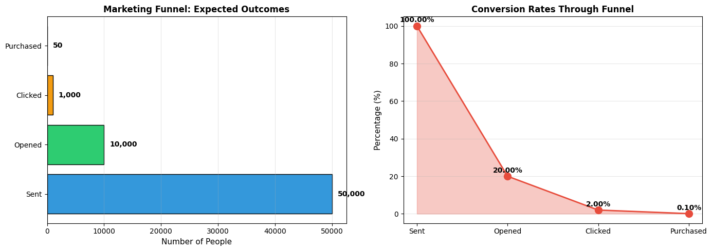
Output:
=== MARKETING FUNNEL ANALYSIS ===
Probability of opening: 20.0%
Probability of NOT opening: 80.0%
Probability of clicking (given open): 10.0%
Probability of purchase (given click): 5.0%
Overall probability of purchase: 0.100%
=== EXPECTED OUTCOMES FROM 50,000 EMAILS ===
Opens: 10,000 (20.0%)
Clicks: 1,000 (2.00%)
Purchases: 50 (0.100%)
Business Insights:
-
Only 0.1% of recipients will purchase
—this might sound low, but it's typical for cold email campaigns
-
The biggest drop-off is at the open stage
—80% never open the email. This suggests:
- Improve subject lines
- Better audience targeting
- Test send times
-
Expected 50 purchases from 50,000 emails
—if average purchase value is $100, that's $5,000 revenue. Compare this to campaign cost to determine ROI.
-
Each stage multiplies probabilities
—small improvements at each stage compound. If you improve open rate from 20% to 25%, purchases increase by 25% (from 50 to 62.5).
4.3.2 Conditional Probability and Bayes' Theorem
Conditional Probability
Conditional probability is the probability of an event occurring, given that another event has already occurred.
Notation : P(A|B) reads as "probability of A given B"
Formula :
P(A|B) = P(A and B) / P(B)
Intuition : We're restricting our attention to only those cases where B occurred, and asking how often A also occurs in those cases.
Example :
In a company:
- 60% of employees are in Sales
- 40% of employees are in Engineering
- 30% of Sales employees have MBA degrees
- 50% of Engineering employees have MBA degrees
Question : If you randomly select an employee with an MBA, what's the probability they're in Engineering?
This is asking: P(Engineering | MBA)
Let's calculate:
Prompt to AI:
Given:
- P(Sales) = 0.60
- P(Engineering) = 0.40
- P(MBA | Sales) = 0.30
- P(MBA | Engineering) = 0.50
Calculate:
1. P(MBA and Sales)
2. P(MBA and Engineering)
3. P(MBA) - total probability of having MBA
4. P(Engineering | MBA) - probability of being in Engineering given MBA
Show the calculations step by step.
Python Code:
# Given probabilities
p_sales = 0.60
p_engineering = 0.40
p_mba_given_sales = 0.30
p_mba_given_engineering = 0.50
# Step 1: Calculate P(MBA and Sales)
p_mba_and_sales = p_sales * p_mba_given_sales
# Step 2: Calculate P(MBA and Engineering)
p_mba_and_engineering = p_engineering * p_mba_given_engineering
# Step 3: Calculate P(MBA) using law of total probability
p_mba = p_mba_and_sales + p_mba_and_engineering
# Step 4: Calculate P(Engineering | MBA) using Bayes' theorem
p_engineering_given_mba = p_mba_and_engineering / p_mba
# Display results
print("=== CONDITIONAL PROBABILITY ANALYSIS ===\n")
print("Given Information:")
print(f" P(Sales) = {p_sales:.0%}")
print(f" P(Engineering) = {p_engineering:.0%}")
print(f" P(MBA | Sales) = {p_mba_given_sales:.0%}")
print(f" P(MBA | Engineering) = {p_mba_given_engineering:.0%}")
print("\nCalculations:")
print(f" P(MBA and Sales) = P(Sales) × P(MBA|Sales)")
print(f" = {p_sales:.2f} × {p_mba_given_sales:.2f} = {p_mba_and_sales:.2f}")
print(f"\n P(MBA and Engineering) = P(Engineering) × P(MBA|Engineering)")
print(f" = {p_engineering:.2f} × {p_mba_given_engineering:.2f} = {p_mba_and_engineering:.2f}")
print(f"\n P(MBA) = P(MBA and Sales) + P(MBA and Engineering)")
print(f" = {p_mba_and_sales:.2f} + {p_mba_and_engineering:.2f} = {p_mba:.2f}")
print(f"\n P(Engineering | MBA) = P(MBA and Engineering) / P(MBA)")
print(f" = {p_mba_and_engineering:.2f} / {p_mba:.2f} = {p_engineering_given_mba:.2f}")
print(f"\n=== ANSWER ===")
print(f"If an employee has an MBA, there's a {p_engineering_given_mba:.1%} chance they're in Engineering")
print(f"and a {1-p_engineering_given_mba:.1%} chance they're in Sales.")
Output:
=== CONDITIONAL PROBABILITY ANALYSIS ===
Given Information:
P(Sales) = 60%
P(Engineering) = 40%
P(MBA | Sales) = 30%
P(MBA | Engineering) = 50%
Calculations:
P(MBA and Sales) = P(Sales) × P(MBA|Sales)
= 0.60 × 0.30 = 0.18
P(MBA and Engineering) = P(Engineering) × P(MBA|Engineering)
= 0.40 × 0.50 = 0.20
P(MBA) = P(MBA and Sales) + P(MBA and Engineering)
= 0.18 + 0.20 = 0.38
P(Engineering | MBA) = P(MBA and Engineering) / P(MBA)
= 0.20 / 0.38 = 0.53
=== ANSWER ===
If an employee has an MBA, there's a 52.6% chance they're in Engineering
and a 47.4% chance they're in Sales.
Key Insight : Even though only 40% of employees are in Engineering, 52.6% of MBA holders are in Engineering. Why? Because Engineering employees are more likely to have MBAs (50% vs. 30%).
This is Bayes' Theorem in action.
Bayes' Theorem
Bayes' Theorem is one of the most important formulas in statistics. It lets us "reverse" conditional probabilities.
Formula :
P(A|B) = [P(B|A) × P(A)] / P(B)
In words:
P(A given B) = [P(B given A) × P(A)] / P(B)
Why it matters : Often we know P(B|A) but want to find P(A|B).
Classic Example: Medical Testing
A disease affects 1% of the population. A test for the disease is 95% accurate (detects disease when present) and has a 5% false positive rate (incorrectly indicates disease when absent).
You test positive. What's the probability you actually have the disease?
Intuition says : 95% (the test accuracy)
Reality : Much lower!
Let's calculate:
Prompt to AI:
Use Bayes' Theorem to solve this medical testing problem:
- P(Disease) = 0.01 (1% of population has disease)
- P(Positive Test | Disease) = 0.95 (test detects 95% of cases)
- P(Positive Test | No Disease) = 0.05 (5% false positive rate)
Calculate P(Disease | Positive Test)
Show all steps and create a visualization.
Python Code:
# Given probabilities
p_disease = 0.01
p_no_disease = 1 - p_disease
p_positive_given_disease = 0.95
p_positive_given_no_disease = 0.05
# Calculate P(Positive Test) using law of total probability
p_positive = (p_positive_given_disease * p_disease +
p_positive_given_no_disease * p_no_disease)
# Apply Bayes' Theorem
p_disease_given_positive = (p_positive_given_disease * p_disease) / p_positive
# Display results
print("=== BAYES' THEOREM: MEDICAL TEST EXAMPLE ===\n")
print("Given:")
print(f" P(Disease) = {p_disease:.1%}")
print(f" P(Positive | Disease) = {p_positive_given_disease:.0%}")
print(f" P(Positive | No Disease) = {p_positive_given_no_disease:.0%}")
print("\nStep 1: Calculate P(Positive Test)")
print(f" P(Positive) = P(Positive|Disease) × P(Disease) + P(Positive|No Disease) × P(No Disease)")
print(f" = {p_positive_given_disease:.2f} × {p_disease:.2f} + {p_positive_given_no_disease:.2f} × {p_no_disease:.2f}")
print(f" = {p_positive_given_disease * p_disease:.4f} + {p_positive_given_no_disease * p_no_disease:.4f}")
print(f" = {p_positive:.4f}")
print("\nStep 2: Apply Bayes' Theorem")
print(f" P(Disease | Positive) = P(Positive|Disease) × P(Disease) / P(Positive)")
print(f" = {p_positive_given_disease:.2f} × {p_disease:.2f} / {p_positive:.4f}")
print(f" = {p_positive_given_disease * p_disease:.4f} / {p_positive:.4f}")
print(f" = {p_disease_given_positive:.4f}")
print(f"\n=== ANSWER ===")
print(f"If you test positive, the probability you actually have the disease is {p_disease_given_positive:.1%}")
print(f"\nThis seems surprisingly low! Here's why:")
print(f" • The disease is rare (only {p_disease:.1%} of people have it)")
print(f" • So most positive tests come from the {p_no_disease:.0%} who don't have it")
print(f" • Even with a low false positive rate ({p_positive_given_no_disease:.0%}), there are many false positives")
# Visualization: Out of 10,000 people
population = 10000
people_with_disease = int(population * p_disease)
people_without_disease = population - people_with_disease
true_positives = int(people_with_disease * p_positive_given_disease)
false_negatives = people_with_disease - true_positives
false_positives = int(people_without_disease * p_positive_given_no_disease)
true_negatives = people_without_disease - false_positives
print(f"\n=== VISUALIZATION: OUT OF {population:,} PEOPLE ===\n")
print(f"Have disease ({p_disease:.1%}): {people_with_disease:>4} people")
print(f" Test Positive (True Positive): {true_positives:>4}")
print(f" Test Negative (False Negative): {false_negatives:>4}")
print(f"\nDon't have disease ({p_no_disease:.0%}): {people_without_disease:>4} people")
print(f" Test Positive (False Positive): {false_positives:>4}")
print(f" Test Negative (True Negative): {true_negatives:>4}")
print(f"\nTotal Positive Tests: {true_positives + false_positives}")
print(f" Of these, {true_positives} actually have disease ({true_positives/(true_positives+false_positives):.1%})")
print(f" And {false_positives} don't have disease ({false_positives/(true_positives+false_positives):.1%})")
# Create visualization
import matplotlib.pyplot as plt
fig, (ax1, ax2) = plt.subplots(1, 2, figsize=(14, 6))
# Population breakdown
categories = ['True\nPositive', 'False\nNegative', 'False\nPositive', 'True\nNegative']
values = [true_positives, false_negatives, false_positives, true_negatives]
colors = ['#2ecc71', '#e74c3c', '#e67e22', '#3498db']
ax1.bar(categories, values, color=colors, edgecolor='black', linewidth=1.5)
for i, (cat, val) in enumerate(zip(categories, values)):
ax1.text(i, val + 50, f'{val:,}', ha='center', fontweight='bold', fontsize=11)
ax1.set_ylabel('Number of People', fontsize=11)
ax1.set_title(f'Test Results for {population:,} People', fontsize=12, fontweight='bold')
ax1.grid(axis='y', alpha=0.3)
# Among positive tests
positive_labels = ['Actually\nHave Disease', 'Actually\nDon\'t Have Disease']
positive_values = [true_positives, false_positives]
positive_colors = ['#2ecc71', '#e67e22']
ax2.bar(positive_labels, positive_values, color=positive_colors, edgecolor='black', linewidth=1.5)
for i, val in enumerate(positive_values):
pct = val / (true_positives + false_positives) * 100
ax2.text(i, val + 10, f'{val}\n({pct:.1f}%)', ha='center', fontweight='bold', fontsize=11)
ax2.set_ylabel('Number of People', fontsize=11)
ax2.set_title('Among Those Who Test Positive', fontsize=12, fontweight='bold')
ax2.grid(axis='y', alpha=0.3)
plt.tight_layout()
plt.show()

Output:
=== BAYES' THEOREM: MEDICAL TEST EXAMPLE ===
Given:
P(Disease) = 1.0%
P(Positive | Disease) = 95%
P(Positive | No Disease) = 5%
Step 1: Calculate P(Positive Test)
P(Positive) = P(Positive|Disease) × P(Disease) + P(Positive|No Disease) × P(No Disease)
= 0.95 × 0.01 + 0.05 × 0.99
= 0.0095 + 0.0495
= 0.0590
Step 2: Apply Bayes' Theorem
P(Disease | Positive) = P(Positive|Disease) × P(Disease) / P(Positive)
= 0.95 × 0.01 / 0.0590
= 0.0095 / 0.0590
= 0.1610
=== ANSWER ===
If you test positive, the probability you actually have the disease is 16.1%
This seems surprisingly low! Here's why:
• The disease is rare (only 1.0% of people have it)
• So most positive tests come from the 99% who don't have it
• Even with a low false positive rate (5%), there are many false positives
=== VISUALIZATION: OUT OF 10,000 PEOPLE ===
Have disease (1.0%): 100 people
Test Positive (True Positive): 95
Test Negative (False Negative): 5
Don't have disease (99%): 9900 people
Test Positive (False Positive): 495
Test Negative (True Negative): 9405
Total Positive Tests: 590
Of these, 95 actually have disease (16.1%)
And 495 don't have disease (83.9%)
This is shocking! Despite a 95% accurate test, if you test positive, there's only a 16.1% chance you actually have the disease.
Why? Because the disease is rare. Out of 10,000 people:
- 100 have the disease → 95 test positive (true positives)
- 9,900 don't have the disease → 495 test positive (false positives)
- Total positive tests: 590
- Only 95 out of 590 (16.1%) actually have the disease
Business Application: Fraud Detection
This same logic applies to fraud detection, spam filtering, and any rare event detection.
If fraud is rare (say, 0.5% of transactions) and your model is 90% accurate, most "fraud alerts" will be false positives. This is why fraud teams need to balance sensitivity (catching fraud) with specificity (not overwhelming investigators with false alarms).
Practical Business Example: Customer Churn Prediction
You're analyzing customer churn. Historical data shows:
- 10% of customers churn each year
- 70% of customers who churn had a support ticket in the last month
- 20% of customers who don't churn had a support ticket in the last month
Question : If a customer has a support ticket, what's the probability they'll churn?
Prompt to AI:
Use Bayes' Theorem:
- P(Churn) = 0.10
- P(Support Ticket | Churn) = 0.70
- P(Support Ticket | No Churn) = 0.20
Calculate P(Churn | Support Ticket) and interpret for business.
Python Code:
# Given probabilities
p_churn = 0.10
p_no_churn = 1 - p_churn
p_ticket_given_churn = 0.70
p_ticket_given_no_churn = 0.20
# Calculate P(Support Ticket)
p_ticket = (p_ticket_given_churn * p_churn +
p_ticket_given_no_churn * p_no_churn)
# Apply Bayes' Theorem
p_churn_given_ticket = (p_ticket_given_churn * p_churn) / p_ticket
print("=== CUSTOMER CHURN ANALYSIS ===\n")
print(f"Base churn rate: {p_churn:.0%}")
print(f"Churn rate among customers with support ticket: {p_churn_given_ticket:.1%}")
print(f"\nIncrease in churn risk: {p_churn_given_ticket/p_churn:.1f}x")
print(f"\n=== BUSINESS INSIGHT ===")
print(f"Customers with support tickets are {p_churn_given_ticket/p_churn:.1f}x more likely to churn.")
print(f"This suggests:")
print(f" • Support tickets indicate customer dissatisfaction")
print(f" • Proactive outreach to these customers could reduce churn")
print(f" • Improving support quality is critical for retention")
# Calculate expected impact of intervention
customers = 10000
customers_with_tickets = int(customers * p_ticket)
expected_churns_with_tickets = int(customers_with_tickets * p_churn_given_ticket)
print(f"\n=== EXPECTED IMPACT ===")
print(f"Out of {customers:,} customers:")
print(f" • {customers_with_tickets:,} will have support tickets")
print(f" • {expected_churns_with_tickets:,} of those will churn")
print(f"\nIf you could reduce churn by 50% among ticket holders:")
print(f" • You'd save {expected_churns_with_tickets//2:,} customers")
print(f" • At $1,000 lifetime value, that's ${expected_churns_with_tickets//2 * 1000:,} in retained revenue")
Output:
=== CUSTOMER CHURN ANALYSIS ===
Base churn rate: 10%
Churn rate among customers with support ticket: 28.0%
Increase in churn risk: 2.8x
=== BUSINESS INSIGHT ===
Customers with support tickets are 2.8x more likely to churn.
This suggests:
• Support tickets indicate customer dissatisfaction
• Proactive outreach to these customers could reduce churn
• Improving support quality is critical for retention
=== EXPECTED IMPACT ===
Out of 10,000 customers:
• 2,500 will have support tickets
• 700 of those will churn
If you could reduce churn by 50% among ticket holders:
• You'd save 350 customers
• At $1,000 lifetime value, that's $350,000 in retained revenue
This is actionable! You now know:
- Support tickets are a strong churn signal
- You can quantify the risk (28% vs. 10% baseline)
- You can estimate the value of intervention ($350,000)
This justifies investing in better support, proactive outreach, or retention campaigns for customers with tickets.
Key Takeaways: Conditional Probability and Bayes' Theorem
-
Conditional probability lets you update beliefs based on new information
-
P(A|B) is not the same as P(B|A)
—don't confuse them!
-
Bayes' Theorem is essential for rare event detection
—medical testing, fraud detection, spam filtering
-
Base rates matter enormously
—a rare event will have many false positives even with an accurate test
-
Business applications are everywhere
—churn prediction, customer segmentation, risk assessment, A/B test analysis
4.4 Common Probability Distributions in Business
Real-world business data often follows recognizable patterns called probability distributions . Understanding these distributions helps you:
- Model uncertainty
- Make predictions
- Calculate probabilities
- Simulate scenarios
We'll cover four distributions that appear constantly in business analytics.
4.4.1 Binomial, Poisson, Normal, Exponential
1. Binomial Distribution
When to use it : Counting successes in a fixed number of independent trials, where each trial has the same probability of success.
Examples:
- Number of customers who buy out of 100 who visit your store
- Number of defective items in a batch of 50
- Number of emails opened out of 1,000 sent
Parameters:
- n : number of trials
- p : probability of success on each trial
Key properties:
- Mean = n × p
- Standard deviation = √(n × p × (1-p))
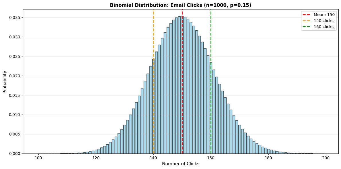
Business Example: Email Campaign
You send 1,000 emails. Historically, 15% of recipients click. What's the probability that exactly 140 people click? What's the probability that at least 160 people click?
Prompt to AI:
Use the binomial distribution with n=1000, p=0.15 to:
1. Calculate probability of exactly 140 clicks
2. Calculate probability of at least 160 clicks
3. Calculate mean and standard deviation
4. Plot the distribution
Python Code:
from scipy import stats
import numpy as np
import matplotlib.pyplot as plt
# Parameters
n = 1000 # number of emails
p = 0.15 # click probability
# Create binomial distribution
binom_dist = stats.binom(n, p)
# Calculate probabilities
prob_exactly_140 = binom_dist.pmf(140)
prob_at_least_160 = 1 - binom_dist.cdf(159) # P(X >= 160) = 1 - P(X <= 159)
# Calculate mean and std
mean = n * p
std = np.sqrt(n * p * (1-p))
print("=== BINOMIAL DISTRIBUTION: EMAIL CLICKS ===\n")
print(f"Parameters: n={n}, p={p:.0%}")
print(f"\nExpected clicks: {mean:.0f}")
print(f"Standard deviation: {std:.1f}")
print(f"\nP(exactly 140 clicks) = {prob_exactly_140:.4f} or {prob_exactly_140:.2%}")
print(f"P(at least 160 clicks) = {prob_at_least_160:.4f} or {prob_at_least_160:.2%}")
# Interpretation
print(f"\n=== INTERPRETATION ===")
print(f"• We expect about {mean:.0f} clicks, give or take {std:.0f}")
print(f"• 140 clicks is {(140-mean)/std:.1f} standard deviations below the mean")
print(f"• 160 clicks is {(160-mean)/std:.1f} standard deviations above the mean")
print(f"• Getting 160+ clicks is unlikely ({prob_at_least_160:.1%} chance)")
# Plot distribution
x = np.arange(100, 200)
pmf = binom_dist.pmf(x)
plt.figure(figsize=(12, 6))
plt.bar(x, pmf, color='skyblue', edgecolor='black', alpha=0.7)
plt.axvline(mean, color='red', linestyle='--', linewidth=2, label=f'Mean: {mean:.0f}')
plt.axvline(140, color='orange', linestyle='--', linewidth=2, label='140 clicks')
plt.axvline(160, color='green', linestyle='--', linewidth=2, label='160 clicks')
plt.xlabel('Number of Clicks', fontsize=11)
plt.ylabel('Probability', fontsize=11)
plt.title('Binomial Distribution: Email Clicks (n=1000, p=0.15)', fontsize=12, fontweight='bold')
plt.legend()
plt.grid(axis='y', alpha=0.3)
plt.tight_layout()
plt.show()
Output:
=== BINOMIAL DISTRIBUTION: EMAIL CLICKS ===
Parameters: n=1000, p=15%
Expected clicks: 150 Standard deviation: 11.3
P(exactly 140 clicks) = 0.0177 or 1.77% P(at least 160 clicks) = 0.1867 or 18.67%
=== INTERPRETATION === • We expect about 150 clicks, give or take 11 • 140 clicks is -0.9 standard deviations below the mean • 160 clicks is 0.9 standard deviations above the mean • Getting 160+ clicks is unlikely (18.7% chance)
Business Application:
If you get 160+ clicks, should you conclude your campaign performed better than usual? Not necessarily—there's an 18.7% chance of getting that many just by random variation. You'd need significantly more (say, 175+) to be confident the campaign truly outperformed.
2. Poisson Distribution
When to use it: Counting events that occur randomly over time or space, when events are independent and the average rate is constant.
Examples:
- Number of customer service calls per hour
- Number of defects per square meter of fabric
- Number of website visits per minute
- Number of accidents per month
Parameter:
- λ (lambda): average rate of events
Key properties:
- Mean = λ
- Standard deviation = √λ
- Variance = λ
Business Example: Customer Service Calls
Your call center receives an average of 12 calls per hour. What's the probability of receiving exactly 15 calls in the next hour? What's the probability of receiving more than 20 calls?
from scipy import stats
import numpy as np
import matplotlib.pyplot as plt
# Parameter
lambda_rate = 12 # average calls per hour
# Create Poisson distribution
poisson_dist = stats.poisson(lambda_rate)
# Calculate probabilities
prob_exactly_15 = poisson_dist.pmf(15)
prob_more_than_20 = 1 - poisson_dist.cdf(20) # P(X > 20) = 1 - P(X <= 20)
prob_fewer_than_8 = poisson_dist.cdf(7) # P(X < 8) = P(X <= 7)
print("=== POISSON DISTRIBUTION: CALL CENTER ===\n")
print(f"Average rate: λ = {lambda_rate} calls/hour")
print(f"Standard deviation: {np.sqrt(lambda_rate):.2f}")
print(f"\nP(exactly 15 calls) = {prob_exactly_15:.4f} or {prob_exactly_15:.2%}")
print(f"P(more than 20 calls) = {prob_more_than_20:.4f} or {prob_more_than_20:.2%}")
print(f"P(fewer than 8 calls) = {prob_fewer_than_8:.4f} or {prob_fewer_than_8:.2%}")
# Staffing implications
print(f"\n=== STAFFING IMPLICATIONS ===")
print(f"• If you staff for 12 calls/hour, you'll be understaffed {1-poisson_dist.cdf(12):.1%} of the time")
print(f"• If you staff for 15 calls/hour, you'll be understaffed {1-poisson_dist.cdf(15):.1%} of the time")
print(f"• If you staff for 18 calls/hour, you'll be understaffed {1-poisson_dist.cdf(18):.1%} of the time")
# Calculate 95th percentile (capacity needed to handle 95% of hours)
capacity_95 = poisson_dist.ppf(0.95)
print(f"\n• To handle 95% of hours, staff for {capacity_95:.0f} calls/hour")
# Plot distribution
x = np.arange(0, 30)
pmf = poisson_dist.pmf(x)
plt.figure(figsize=(12, 6))
plt.bar(x, pmf, color='lightcoral', edgecolor='black', alpha=0.7)
plt.axvline(lambda_rate, color='red', linestyle='--', linewidth=2, label=f'Mean: {lambda_rate}')
plt.axvline(capacity_95, color='green', linestyle='--', linewidth=2, label=f'95th percentile: {capacity_95:.0f}')
plt.xlabel('Number of Calls per Hour', fontsize=11)
plt.ylabel('Probability', fontsize=11)
plt.title(f'Poisson Distribution: Call Arrivals (λ={lambda_rate})', fontsize=12, fontweight='bold')
plt.legend()
plt.grid(axis='y', alpha=0.3)
plt.tight_layout()
plt.show()

Output:
=== POISSON DISTRIBUTION: CALL CENTER ===
Average rate: λ = 12 calls/hour
Standard deviation: 3.46
P(exactly 15 calls) = 0.0724 or 7.24%
P(more than 20 calls) = 0.0046 or 0.46%
P(fewer than 8 calls) = 0.0895 or 8.95%
=== STAFFING IMPLICATIONS ===
• If you staff for 12 calls/hour, you'll be understaffed 57.7% of the time
• If you staff for 15 calls/hour, you'll be understaffed 22.4% of the time
• If you staff for 18 calls/hour, you'll be understaffed 4.2% of the time
• To handle 95% of hours, staff for 18 calls/hour
Business Insight:
Even though the average is 12 calls/hour, you need to staff for 18 calls/hour to handle 95% of hours. This is the nature of random variation—you need capacity above the average to handle peaks.
3. Normal Distribution (Gaussian)
When to use it : Continuous data that clusters around a mean, with symmetric tails. The most important distribution in statistics.
Examples:
- Heights, weights
- Test scores
- Measurement errors
- Many business metrics (when aggregated)
Parameters:
- μ (mu) : mean
- σ (sigma) : standard deviation
Key properties:
- Bell-shaped, symmetric
- 68% of data within ±1 standard deviation of mean
- 95% of data within ±2 standard deviations
- 99.7% of data within ±3 standard deviations
The Central Limit Theorem : Even if individual data points aren't normally distributed, averages of large samples tend to be normally distributed. This is why the normal distribution is so important.
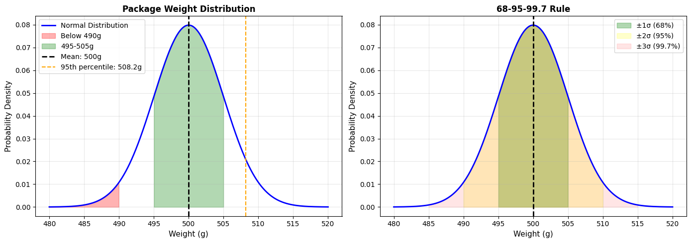
Business Example: Product Weights
Your factory produces packages with a target weight of 500g. The actual weight follows a normal distribution with mean 500g and standard deviation 5g.
What percentage of packages weigh less than 490g? What weight represents the 95th percentile?
Prompt to AI:
Use the normal distribution with μ=500, σ=5 to:
1. Calculate percentage below 490g
2. Calculate percentage between 495g and 505g
3. Find the 95th percentile weight
4. Plot the distribution with shaded regions
Python Code:
from scipy import stats
import numpy as np
import matplotlib.pyplot as plt
# Parameters
mu = 500 # mean weight (g)
sigma = 5 # standard deviation (g)
# Create normal distribution
normal_dist = stats.norm(mu, sigma)
# Calculate probabilities
prob_below_490 = normal_dist.cdf(490)
prob_between_495_505 = normal_dist.cdf(505) - normal_dist.cdf(495)
percentile_95 = normal_dist.ppf(0.95)
print("=== NORMAL DISTRIBUTION: PACKAGE WEIGHTS ===\n")
print(f"Mean: μ = {mu}g")
print(f"Standard Deviation: σ = {sigma}g")
print(f"\nP(weight < 490g) = {prob_below_490:.4f} or {prob_below_490:.2%}")
print(f"P(495g < weight < 505g) = {prob_between_495_505:.4f} or {prob_between_495_505:.2%}")
print(f"95th percentile weight = {percentile_95:.2f}g")
# Quality control implications
print(f"\n=== QUALITY CONTROL ===")
print(f"• {prob_below_490:.2%} of packages are more than 2σ below target")
print(f"• {prob_between_495_505:.2%} of packages are within ±1σ of target")
# Calculate percentage outside specification limits
spec_lower = 485
spec_upper = 515
prob_out_of_spec = prob_below_490 + (1 - normal_dist.cdf(spec_upper))
print(f"\nIf specification limits are {spec_lower}g to {spec_upper}g:")
print(f"• {normal_dist.cdf(spec_lower):.4%} are below {spec_lower}g")
print(f"• {1-normal_dist.cdf(spec_upper):.4%} are above {spec_upper}g")
print(f"• {(normal_dist.cdf(spec_lower) + (1-normal_dist.cdf(spec_upper))):.2%} are out of specification")
# Plot distribution
x = np.linspace(mu - 4*sigma, mu + 4*sigma, 1000)
y = normal_dist.pdf(x)
fig, (ax1, ax2) = plt.subplots(1, 2, figsize=(14, 5))
# Plot 1: Show key regions
ax1.plot(x, y, 'b-', linewidth=2, label='Normal Distribution')
ax1.fill_between(x, y, where=(x < 490), color='red', alpha=0.3, label='Below 490g')
ax1.fill_between(x, y, where=((x >= 495) & (x <= 505)), color='green', alpha=0.3, label='495-505g')
ax1.axvline(mu, color='black', linestyle='--', linewidth=2, label=f'Mean: {mu}g')
ax1.axvline(percentile_95, color='orange', linestyle='--', linewidth=1.5, label=f'95th percentile: {percentile_95:.1f}g')
ax1.set_xlabel('Weight (g)', fontsize=11)
ax1.set_ylabel('Probability Density', fontsize=11)
ax1.set_title('Package Weight Distribution', fontsize=12, fontweight='bold')
ax1.legend()
ax1.grid(alpha=0.3)
# Plot 2: Show 68-95-99.7 rule
ax2.plot(x, y, 'b-', linewidth=2)
ax2.fill_between(x, y, where=((x >= mu-sigma) & (x <= mu+sigma)),
color='green', alpha=0.3, label='±1σ (68%)')
ax2.fill_between(x, y, where=((x >= mu-2*sigma) & (x <= mu+2*sigma)),
color='yellow', alpha=0.2, label='±2σ (95%)')
ax2.fill_between(x, y, where=((x >= mu-3*sigma) & (x <= mu+3*sigma)),
color='red', alpha=0.1, label='±3σ (99.7%)')
ax2.axvline(mu, color='black', linestyle='--', linewidth=2)
ax2.set_xlabel('Weight (g)', fontsize=11)
ax2.set_ylabel('Probability Density', fontsize=11)
ax2.set_title('68-95-99.7 Rule', fontsize=12, fontweight='bold')
ax2.legend()
ax2.grid(alpha=0.3)
plt.tight_layout()
plt.show()
Output:
=== NORMAL DISTRIBUTION: PACKAGE WEIGHTS ===
Mean: μ = 500g
Standard Deviation: σ = 5g
P(weight < 490g) = 0.0228 or 2.28%
P(495g < weight < 505g) = 0.6827 or 68.27%
95th percentile weight = 508.22g
=== QUALITY CONTROL ===
• 2.28% of packages are more than 2σ below target
• 68.27% of packages are within ±1σ of target
If specification limits are 485g to 515g:
• 0.0013% are below 485g
• 0.0013% are above 515g
• 0.0027% are out of specification
Business Application:
This tells you:
- Your process is well-controlled (only 0.0027% out of spec)
- 2.28% of packages are "light" (below 490g), which might concern customers
- You could tighten quality control by reducing σ (less variation)
4. Exponential Distribution
When to use it : Modeling time between events in a Poisson process.
Examples:
- Time between customer arrivals
- Time until equipment failure
- Time between purchases
- Duration of phone calls
Parameter:
- λ (lambda) : rate parameter (events per unit time)
- Mean time between events = 1/λ
Key property:
- "Memoryless" property: The probability of an event in the next time period doesn't depend on how long you've already waited
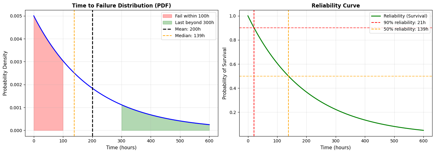
Business Example: Equipment Maintenance
A machine fails on average once every 200 hours (λ = 1/200 = 0.005 failures per hour). What's the probability it fails within the next 100 hours? What's the probability it lasts more than 300 hours?
Prompt to AI:
Use the exponential distribution with mean=200 hours to:
1. Calculate probability of failure within 100 hours
2. Calculate probability of lasting more than 300 hours
3. Find the median time to failure
4. Plot the distribution
Python Code:
from scipy import stats
import numpy as np
import matplotlib.pyplot as plt
# Parameters
mean_time = 200 # mean time between failures (hours)
lambda_rate = 1 / mean_time # rate parameter
# Create exponential distribution
exp_dist = stats.expon(scale=mean_time) # scale = 1/λ = mean
# Calculate probabilities
prob_fail_within_100 = exp_dist.cdf(100)
prob_last_more_than_300 = 1 - exp_dist.cdf(300)
median_time = exp_dist.median()
print("=== EXPONENTIAL DISTRIBUTION: EQUIPMENT FAILURE ===\n")
print(f"Mean time between failures: {mean_time} hours")
print(f"Rate: λ = {lambda_rate:.4f} failures/hour")
print(f"\nP(failure within 100 hours) = {prob_fail_within_100:.4f} or {prob_fail_within_100:.2%}")
print(f"P(lasts more than 300 hours) = {prob_last_more_than_300:.4f} or {prob_last_more_than_300:.2%}")
print(f"Median time to failure = {median_time:.1f} hours")
# Maintenance planning
print(f"\n=== MAINTENANCE PLANNING ===")
for hours in [50, 100, 150, 200, 250]:
prob_survive = 1 - exp_dist.cdf(hours)
print(f"• Probability of surviving {hours:3d} hours: {prob_survive:.2%}")
# Calculate time for 90% reliability
time_90_reliability = exp_dist.ppf(0.10) # 10% failure = 90% survival
print(f"\n• For 90% reliability, perform maintenance every {time_90_reliability:.0f} hours")
# Plot distribution
x = np.linspace(0, 600, 1000)
y = exp_dist.pdf(x)
cdf_y = exp_dist.cdf(x)
fig, (ax1, ax2) = plt.subplots(1, 2, figsize=(14, 5))
ax1.plot(x, y, 'b-', linewidth=2)
ax1.fill_between(x, y, where=(x <= 100), color='red', alpha=0.3, label='Fail within 100h')
ax1.fill_between(x, y, where=(x >= 300), color='green', alpha=0.3, label='Last beyond 300h')
ax1.axvline(mean_time, color='black', linestyle='--', linewidth=2, label=f'Mean: {mean_time}h')
ax1.axvline(median_time, color='orange', linestyle='--', linewidth=1.5, label=f'Median: {median_time:.0f}h')
ax1.set_xlabel('Time (hours)', fontsize=11)
ax1.set_ylabel('Probability Density', fontsize=11)
ax1.set_title('Time to Failure Distribution (PDF)', fontsize=12, fontweight='bold')
ax1.legend()
ax1.grid(alpha=0.3)
# CDF (Reliability curve)
ax2.plot(x, 1-cdf_y, 'g-', linewidth=2, label='Reliability (Survival)')
ax2.axhline(0.90, color='red', linestyle='--', linewidth=1.5, alpha=0.7)
ax2.axvline(time_90_reliability, color='red', linestyle='--', linewidth=1.5,
label=f'90% reliability: {time_90_reliability:.0f}h')
ax2.axhline(0.50, color='orange', linestyle='--', linewidth=1.5, alpha=0.7)
ax2.axvline(median_time, color='orange', linestyle='--', linewidth=1.5,
label=f'50% reliability: {median_time:.0f}h')
ax2.set_xlabel('Time (hours)', fontsize=11)
ax2.set_ylabel('Probability of Survival', fontsize=11)
ax2.set_title('Reliability Curve', fontsize=12, fontweight='bold')
ax2.legend()
ax2.grid(alpha=0.3)
plt.tight_layout()
plt.show()
Output:
=== EXPONENTIAL DISTRIBUTION: EQUIPMENT FAILURE ===
Mean time between failures: 200 hours
Rate: λ = 0.0050 failures/hour
P(failure within 100 hours) = 0.3935 or 39.35%
P(lasts more than 300 hours) = 0.2231 or 22.31%
Median time to failure = 138.6 hours
=== MAINTENANCE PLANNING ===
• Probability of surviving 50 hours: 77.88%
• Probability of surviving 100 hours: 60.65%
• Probability of surviving 150 hours: 47.24%
• Probability of surviving 200 hours: 36.79%
• Probability of surviving 250 hours: 28.65%
• For 90% reliability, perform maintenance every 21 hours
Business Insight:
Notice the median (138.6 hours) is less than the mean (200 hours). This is because the exponential distribution is right-skewed—most failures happen relatively early, but a few machines last much longer, pulling the mean up.
For maintenance planning: If you want 90% reliability, you need to perform preventive maintenance every 21 hours, even though the average time to failure is 200 hours. This is the cost of high reliability.
4.4.2 Applications in Demand, Risk, and Reliability
Let's see how these distributions apply to real business problems.
Application 1: Demand Forecasting
Scenario : A retailer needs to decide how much inventory to stock. Daily demand follows a normal distribution with mean 100 units and standard deviation 20 units.
Question : How much should they stock to meet demand 95% of the time?
Prompt to AI:
Daily demand: Normal(μ=100, σ=20)
Calculate the inventory level needed for 95% service level.
Also calculate expected stockouts and excess inventory.
Python Code:
from scipy import stats
import numpy as np
# Demand distribution
mu_demand = 100
sigma_demand = 20
demand_dist = stats.norm(mu_demand, sigma_demand)
# Calculate inventory for different service levels
service_levels = [0.80, 0.90, 0.95, 0.99]
print("=== INVENTORY PLANNING ===\n")
print(f"Daily demand: Normal(μ={mu_demand}, σ={sigma_demand})")
print(f"\nService Level Inventory Needed Safety Stock")
print("-" * 50)
for sl in service_levels:
inventory = demand_dist.ppf(sl)
safety_stock = inventory - mu_demand
print(f" {sl:.0%} {inventory:>6.0f} {safety_stock:>+6.0f}")
# Detailed analysis for 95% service level
inventory_95 = demand_dist.ppf(0.95)
safety_stock_95 = inventory_95 - mu_demand
print(f"\n=== 95% SERVICE LEVEL ANALYSIS ===")
print(f"Stock level: {inventory_95:.0f} units")
print(f"Safety stock: {safety_stock_95:.0f} units (buffer above mean)")
# Calculate expected outcomes
prob_stockout = 1 - 0.95
expected_demand_when_stockout = mu_demand + sigma_demand * stats.norm.pdf(stats.norm.ppf(0.95)) / (1 - 0.95)
expected_stockout_units = (expected_demand_when_stockout - inventory_95) * prob_stockout
print(f"\nExpected outcomes:")
print(f"• Stockout probability: {prob_stockout:.1%}")
print(f"• When demand exceeds {inventory_95:.0f}, average demand is {expected_demand_when_stockout:.0f}")
print(f"• Expected lost sales per day: {expected_stockout_units:.1f} units")
# Cost analysis
holding_cost_per_unit = 2 # $ per unit per day
stockout_cost_per_unit = 10 # $ per lost sale
expected_holding_cost = safety_stock_95 * holding_cost_per_unit
expected_stockout_cost = expected_stockout_units * stockout_cost_per_unit
total_expected_cost = expected_holding_cost + expected_stockout_cost
print(f"\n=== COST ANALYSIS ===")
print(f"Holding cost: ${holding_cost_per_unit}/unit/day")
print(f"Stockout cost: ${stockout_cost_per_unit}/unit")
print(f"\nExpected daily costs:")
print(f"• Holding cost: ${expected_holding_cost:.2f}")
print(f"• Stockout cost: ${expected_stockout_cost:.2f}")
print(f"• Total: ${total_expected_cost:.2f}")
Output:
=== INVENTORY PLANNING ===
Daily demand: Normal(μ=100, σ=20)
Service Level Inventory Needed Safety Stock
--------------------------------------------------
80% 117 +17
90% 126 +26
95% 133 +33
99% 147 +47
=== 95% SERVICE LEVEL ANALYSIS ===
Stock level: 133 units
Safety stock: 33 units (buffer above mean)
Expected outcomes:
• Stockout probability: 5.0%
• When demand exceeds 133, average demand is 153
• Expected lost sales per day: 1.0 units
=== COST ANALYSIS ===
Holding cost: \$2/unit/day
Stockout cost: \$10/unit
Expected daily costs:
• Holding cost: \$66.00
• Stockout cost: \$10.00
• Total: \$76.00
Business Decision:
You can now compare different service levels:
- 95% service level: Stock 133 units, total cost $76/day
- 90% service level: Stock 126 units, lower holding cost but more stockouts
- 99% service level: Stock 147 units, almost no stockouts but high holding cost
The optimal choice depends on your specific holding and stockout costs.
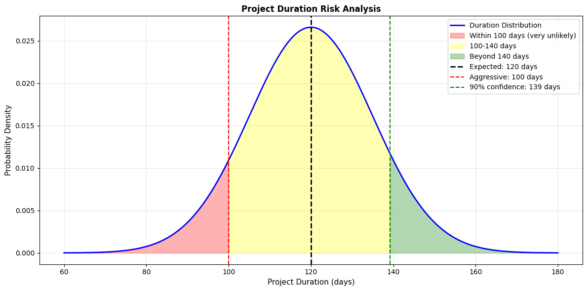
Application 2: Risk Assessment
Scenario : A project has uncertain completion time. Based on historical data, similar projects follow a normal distribution with mean 120 days and standard deviation 15 days.
Question : What's the probability of finishing within 100 days? What deadline should you commit to if you want 90% confidence?
Prompt to AI:
Project duration: Normal(μ=120, σ=15)
Calculate:
1. Probability of finishing within 100 days
2. Deadline for 90% confidence
3. Create a risk visualization
Python Code:
from scipy import stats
import numpy as np
import matplotlib.pyplot as plt
# Project duration distribution
mu_duration = 120 # days
sigma_duration = 15 # days
duration_dist = stats.norm(mu_duration, sigma_duration)
# Calculate probabilities
prob_within_100 = duration_dist.cdf(100)
deadline_90_confidence = duration_dist.ppf(0.90)
deadline_95_confidence = duration_dist.ppf(0.95)
print("=== PROJECT RISK ANALYSIS ===\n")
print(f"Expected duration: {mu_duration} days")
print(f"Standard deviation: {sigma_duration} days")
print(f"\nP(finish within 100 days) = {prob_within_100:.2%}")
print(f" → This is {(mu_duration - 100)/sigma_duration:.1f} standard deviations below the mean")
print(f" → Very unlikely!")
print(f"\nRecommended deadlines:")
print(f"• 50% confidence: {mu_duration:.0f} days (expected duration)")
print(f"• 90% confidence: {deadline_90_confidence:.0f} days")
print(f"• 95% confidence: {deadline_95_confidence:.0f} days")
# Risk table
print(f"\n=== RISK TABLE ===")
print(f"Deadline Probability Risk Level")
print("-" * 45)
deadlines = [100, 110, 120, 130, 140, 150]
for d in deadlines:
prob = duration_dist.cdf(d)
risk = 1 - prob
risk_level = "VERY HIGH" if risk > 0.3 else "HIGH" if risk > 0.1 else "MEDIUM" if risk > 0.05 else "LOW"
print(f"{d:3d} days {prob:>5.1%} {risk_level}")
# Visualization
x = np.linspace(mu_duration - 4*sigma_duration, mu_duration + 4*sigma_duration, 1000)
y = duration_dist.pdf(x)
plt.figure(figsize=(12, 6))
plt.plot(x, y, 'b-', linewidth=2, label='Duration Distribution')
# Shade regions
plt.fill_between(x, y, where=(x <= 100), color='red', alpha=0.3, label='Within 100 days (very unlikely)')
plt.fill_between(x, y, where=((x > 100) & (x <= deadline_90_confidence)),
color='yellow', alpha=0.3, label='100-140 days')
plt.fill_between(x, y, where=(x > deadline_90_confidence),
color='green', alpha=0.3, label='Beyond 140 days')
# Add reference lines
plt.axvline(mu_duration, color='black', linestyle='--', linewidth=2, label=f'Expected: {mu_duration} days')
plt.axvline(100, color='red', linestyle='--', linewidth=1.5, label='Aggressive: 100 days')
plt.axvline(deadline_90_confidence, color='green', linestyle='--', linewidth=1.5,
label=f'90% confidence: {deadline_90_confidence:.0f} days')
plt.xlabel('Project Duration (days)', fontsize=11)
plt.ylabel('Probability Density', fontsize=11)
plt.title('Project Duration Risk Analysis', fontsize=12, fontweight='bold')
plt.legend()
plt.grid(alpha=0.3)
plt.tight_layout()
plt.show()
Output:
=== PROJECT RISK ANALYSIS ===
Expected duration: 120 days
Standard deviation: 15 days
P(finish within 100 days) = 9.12%
→ This is -1.3 standard deviations below the mean
→ Very unlikely!
Recommended deadlines:
• 50% confidence: 120 days (expected duration)
• 90% confidence: 139 days
• 95% confidence: 145 days
=== RISK TABLE ===
Deadline Probability Risk Level
---------------------------------------------
100 days 9.1% VERY HIGH
110 days 25.2% VERY HIGH
120 days 50.0% VERY HIGH
130 days 74.8% HIGH
140 days 90.9% MEDIUM
150 days 97.7% LOW
Business Communication:
When your manager asks "Can we finish in 100 days?", you can now say:
"Based on historical data, there's only a 9% chance of finishing within 100 days. I recommend committing to 140 days, which gives us 90% confidence. If we absolutely must commit to 100 days, we need to understand we'll likely miss that deadline and should plan contingencies."
This is much better than saying "I think so" or "probably not."
Application 3: Reliability Engineering
Scenario : You're evaluating two suppliers for a critical component.
- Supplier A : Components fail following exponential distribution with mean time to failure = 1000 hours
- Supplier B : Components fail following exponential distribution with mean time to failure = 1500 hours, but cost 30% more
Question : Which supplier offers better value?
Prompt to AI:
Compare two suppliers:
- Supplier A: MTTF = 1000 hours, cost = \$100
- Supplier B: MTTF = 1500 hours, cost = \$130
Calculate:
1. Reliability at 500, 1000, 1500 hours
2. Expected number of failures over 5000 hours
3. Total cost of ownership
Python Code:
from scipy import stats
import numpy as np
import matplotlib.pyplot as plt
# Supplier parameters
mttf_a = 1000 # hours
mttf_b = 1500 # hours
cost_a = 100 # $
cost_b = 130 # $
# Create distributions
dist_a = stats.expon(scale=mttf_a)
dist_b = stats.expon(scale=mttf_b)
# Calculate reliability at key timepoints
timepoints = [500, 1000, 1500, 2000]
print("=== SUPPLIER RELIABILITY COMPARISON ===\n")
print(f"Supplier A: MTTF = {mttf_a}h, Cost = ${cost_a}")
print(f"Supplier B: MTTF = {mttf_b}h, Cost = ${cost_b} (+{(cost_b/cost_a-1)*100:.0f}%)")
print(f"\nReliability (Probability of Survival):")
print(f"Time (hours) Supplier A Supplier B Advantage")
print("-" * 55)
for t in timepoints:
rel_a = 1 - dist_a.cdf(t)
rel_b = 1 - dist_b.cdf(t)
advantage = "B" if rel_b > rel_a else "A"
print(f" {t:>4} {rel_a:>5.1%} {rel_b:>5.1%} {advantage} (+{abs(rel_b-rel_a):.1%})")
# Calculate expected failures over 5000 hours
operating_hours = 5000
expected_failures_a = operating_hours / mttf_a
expected_failures_b = operating_hours / mttf_b
print(f"\n=== TOTAL COST OF OWNERSHIP (5000 hours) ===\n")
# Assume replacement cost = component cost
total_cost_a = cost_a * expected_failures_a
total_cost_b = cost_b * expected_failures_b
print(f"Supplier A:")
print(f" Expected failures: {expected_failures_a:.1f}")
print(f" Total cost: ${total_cost_a:.2f}")
print(f" Cost per hour: ${total_cost_a/operating_hours:.3f}")
print(f"\nSupplier B:")
print(f" Expected failures: {expected_failures_b:.1f}")
print(f" Total cost: ${total_cost_b:.2f}")
print(f" Cost per hour: ${total_cost_b/operating_hours:.3f}")
print(f"\n=== RECOMMENDATION ===")
if total_cost_a < total_cost_b:
savings = total_cost_b - total_cost_a
print(f"Choose Supplier A - saves ${savings:.2f} over 5000 hours ({savings/total_cost_b*100:.1f}%)")
else:
savings = total_cost_a - total_cost_b
print(f"Choose Supplier B - saves ${savings:.2f} over 5000 hours ({savings/total_cost_a*100:.1f}%)")
# Visualization
x = np.linspace(0, 3000, 1000)
reliability_a = 1 - dist_a.cdf(x)
reliability_b = 1 - dist_b.cdf(x)
plt.figure(figsize=(12, 6))
plt.plot(x, reliability_a, 'b-', linewidth=2, label=f'Supplier A (MTTF={mttf_a}h, ${cost_a})')
plt.plot(x, reliability_b, 'g-', linewidth=2, label=f'Supplier B (MTTF={mttf_b}h, ${cost_b})')
# Add reference lines
for t in [500, 1000, 1500]:
plt.axvline(t, color='gray', linestyle=':', alpha=0.5)
plt.axhline(0.5, color='red', linestyle='--', alpha=0.5, label='50% reliability')
plt.xlabel('Operating Hours', fontsize=11)
plt.ylabel('Reliability (Probability of Survival)', fontsize=11)
plt.title('Supplier Reliability Comparison', fontsize=12, fontweight='bold')
plt.legend()
plt.grid(alpha=0.3)
plt.tight_layout()
plt.show()
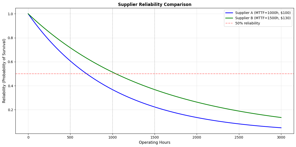
Output:
=== SUPPLIER RELIABILITY COMPARISON ===
Supplier A: MTTF = 1000h, Cost = \$100
Supplier B: MTTF = 1500h, Cost = \$130 (+30%)
Reliability (Probability of Survival):
Time (hours) Supplier A Supplier B Advantage
-------------------------------------------------------
500 60.7% 71.7% B (+11.1%)
1000 36.8% 51.3% B (+14.5%)
1500 22.3% 36.8% B (+14.5%)
2000 13.5% 26.4% B (+12.9%)
=== TOTAL COST OF OWNERSHIP (5000 hours) ===
Supplier A:
Expected failures: 5.0
Total cost: \$500.00
Cost per hour: \$0.100
Supplier B:
Expected failures: 3.3
Total cost: \$433.33
Cost per hour: \$0.087
=== RECOMMENDATION ===
Choose Supplier B - saves \$66.67 over 5000 hours (13.3%)
Business Insight:
Even though Supplier B costs 30% more per component, they're actually cheaper in the long run because you replace them less frequently. Supplier B saves $66.67 (13.3%) over 5000 hours of operation.
This is a classic example of why you need to consider total cost of ownership , not just purchase price.
4.5 Statistical Inference
Descriptive statistics and probability tell us about data we have. Statistical inference lets us draw conclusions about populations based on samples.
This is crucial in business because we almost never have complete data:
- We survey 1,000 customers, not all 1 million
- We test a new feature with 10,000 users, not all 50 million
- We analyze last quarter's sales, not future sales
The fundamental question of inference : What can we confidently say about the whole population based on our sample?
4.5.1 Sampling and Sampling Distributions
Population vs. Sample
- Population : The entire group you want to understand (all customers, all transactions, all products)
- Sample : A subset of the population you actually observe
- Parameter : A numerical characteristic of the population (e.g., population mean μ)
- Statistic : A numerical characteristic of the sample (e.g., sample mean x̄)
Example:
- Population: All 1 million customers
- Sample: 1,000 randomly selected customers
- Parameter: True average customer satisfaction (unknown)
- Statistic: Average satisfaction in our sample of 1,000 (known)
The Challenge:
The sample mean (x̄) is our best estimate of the population mean (μ), but it won't be exactly right. If we took a different sample, we'd get a different sample mean.
Question : How much does the sample mean vary? How confident can we be that it's close to the true population mean?
Answer : The sampling distribution tells us.
Sampling Distribution
If you took many samples and calculated the mean of each, those sample means would form a distribution called the sampling distribution of the mean .
Key facts (from the Central Limit Theorem):
- The sampling distribution is approximately normal (even if the population isn't)
- The mean of the sampling distribution equals the population mean (μ)
- The standard deviation of the sampling distribution (called standard error ) is:
SE = σ / √n
Where:
- σ = population standard deviation
- n = sample size
What this means:
- Larger samples (bigger n) give more precise estimates (smaller SE)
- The sample mean is typically within about 2 standard errors of the true population mean
Practical Example: Customer Satisfaction
You survey 100 customers and find mean satisfaction = 7.2 (on a 1-10 scale) with standard deviation = 1.5.
What can you say about the true average satisfaction of all customers?
Prompt to AI:
Sample: n=100, mean=7.2, SD=1.5
Calculate:
1. Standard error
2. Likely range for true population mean
3. Visualize sampling distribution
Python Code:
from scipy import stats
import numpy as np
import matplotlib.pyplot as plt
# Sample statistics
n = 100
sample_mean = 7.2
sample_sd = 1.5
# Calculate standard error
se = sample_sd / np.sqrt(n)
print("=== SAMPLING DISTRIBUTION ANALYSIS ===\n")
print(f"Sample size: n = {n}")
print(f"Sample mean: x̄ = {sample_mean}")
print(f"Sample SD: s = {sample_sd}")
print(f"Standard error: SE = {se:.3f}")
print(f"\n=== INTERPRETATION ===")
print(f"The true population mean is likely within:")
print(f" • ±1 SE: {sample_mean - se:.2f} to {sample_mean + se:.2f} (68% confidence)")
print(f" • ±2 SE: {sample_mean - 2*se:.2f} to {sample_mean + 2*se:.2f} (95% confidence)")
print(f" • ±3 SE: {sample_mean - 3*se:.2f} to {sample_mean + 3*se:.2f} (99.7% confidence)")
# Simulate sampling distribution
np.random.seed(42)
num_samples = 10000
sample_means = []
# Simulate taking many samples
for _ in range(num_samples):
# Generate a sample (assuming population mean = 7.2, SD = 1.5)
sample = np.random.normal(sample_mean, sample_sd, n)
sample_means.append(np.mean(sample))
sample_means = np.array(sample_means)
# Plot
fig, (ax1, ax2) = plt.subplots(1, 2, figsize=(14, 5))
# Histogram of sample means
ax1.hist(sample_means, bins=50, density=True, color='skyblue', edgecolor='black', alpha=0.7)
# Overlay theoretical normal distribution
x = np.linspace(sample_mean - 4*se, sample_mean + 4*se, 1000)
y = stats.norm.pdf(x, sample_mean, se)
ax1.plot(x, y, 'r-', linewidth=2, label='Theoretical')
ax1.axvline(sample_mean, color='black', linestyle='--', linewidth=2, label=f'Mean: {sample_mean}')
ax1.axvline(sample_mean - 2*se, color='green', linestyle='--', linewidth=1.5, alpha=0.7)
ax1.axvline(sample_mean + 2*se, color='green', linestyle='--', linewidth=1.5, alpha=0.7, label='±2 SE')
ax1.set_xlabel('Sample Mean', fontsize=11)
ax1.set_ylabel('Density', fontsize=11)
ax1.set_title('Sampling Distribution of the Mean', fontsize=12, fontweight='bold')
ax1.legend()
ax1.grid(alpha=0.3)
# Show effect of sample size
sample_sizes = [10, 30, 100, 300]
ax2.set_xlabel('Sample Mean', fontsize=11)
ax2.set_ylabel('Density', fontsize=11)
ax2.set_title('Effect of Sample Size on Standard Error', fontsize=12, fontweight='bold')
for n_size in sample_sizes:
se_size = sample_sd / np.sqrt(n_size)
x = np.linspace(sample_mean - 4*se_size, sample_mean + 4*se_size, 1000)
y = stats.norm.pdf(x, sample_mean, se_size)
ax2.plot(x, y, linewidth=2, label=f'n={n_size}, SE={se_size:.3f}')
ax2.axvline(sample_mean, color='black', linestyle='--', linewidth=1, alpha=0.5)
ax2.legend()
ax2.grid(alpha=0.3)
plt.tight_layout()
plt.show()
print(f"\n=== KEY INSIGHT ===")
print(f"Increasing sample size reduces standard error:")
for n_size in [10, 30, 100, 300, 1000]:
se_size = sample_sd / np.sqrt(n_size)
print(f" n={n_size:>4}: SE = {se_size:.3f}")

Output:
=== SAMPLING DISTRIBUTION ANALYSIS ===
Sample size: n = 100
Sample mean: x̄ = 7.2
Sample SD: s = 1.5
Standard error: SE = 0.150
=== INTERPRETATION ===
The true population mean is likely within:
• ±1 SE: 7.05 to 7.35 (68% confidence)
• ±2 SE: 6.90 to 7.50 (95% confidence)
• ±3 SE: 6.75 to 7.65 (99.7% confidence)
=== KEY INSIGHT ===
Increasing sample size reduces standard error:
n= 10: SE = 0.474
n= 30: SE = 0.274
n= 100: SE = 0.150
n= 300: SE = 0.087
n=1000: SE = 0.047
Business Insight:
With n=100, you can be 95% confident the true average satisfaction is between 6.90 and 7.50. That's a fairly narrow range!
If you need more precision, you'd need a larger sample. Quadrupling the sample size (to 400) would cut the standard error in half.
4.5.2 Confidence Intervals and Hypothesis Testing
Confidence Intervals
A confidence interval gives a range of plausible values for a population parameter.
Formula for confidence interval for a mean:
x̄ ± (critical value) × SE
For a 95% confidence interval:
x̄ ± 1.96 × SE (when n is large)
x̄ ± t* × SE (when n is small, use t-distribution)
Interpretation:
"We are 95% confident that the true population mean is between [lower bound] and [upper bound]."
What "95% confident" means:
If we repeated this process many times (take a sample, calculate a confidence interval), about 95% of those intervals would contain the true population mean.
It does NOT mean "there's a 95% probability the true mean is in this interval." The true mean is fixed (we just don't know it); the interval is what's random.
Practical Example: A/B Test
You're testing two website designs:
- Version A (current): 1,000 visitors, 32 conversions (3.2%)
- Version B (new): 1,000 visitors, 38 conversions (3.8%)
Is Version B really better, or could this be just random variation?
Prompt to AI:
A/B test data:
- Version A: 32/1000 = 3.2% conversion
- Version B: 38/1000 = 3.8% conversion
Calculate:
1. Confidence intervals for each version
2. Confidence interval for the difference
3. Determine if the difference is statistically significant
Python Code:
from scipy import stats
import numpy as np
# Data
n_a = 1000
conversions_a = 32
rate_a = conversions_a / n_a
n_b = 1000
conversions_b = 38
rate_b = conversions_b / n_b
# Standard errors (for proportions: SE = sqrt(p*(1-p)/n))
se_a = np.sqrt(rate_a * (1 - rate_a) / n_a)
se_b = np.sqrt(rate_b * (1 - rate_b) / n_b)
# 95% confidence intervals
z_critical = 1.96 # for 95% confidence
ci_a_lower = rate_a - z_critical * se_a
ci_a_upper = rate_a + z_critical * se_a
ci_b_lower = rate_b - z_critical * se_b
ci_b_upper = rate_b + z_critical * se_b
print("=== A/B TEST ANALYSIS ===\n")
print(f"Version A: {conversions_a}/{n_a} = {rate_a:.1%}")
print(f" 95% CI: [{ci_a_lower:.2%}, {ci_a_upper:.2%}]")
print(f"\nVersion B: {conversions_b}/{n_b} = {rate_b:.1%}")
print(f" 95% CI: [{ci_b_lower:.2%}, {ci_b_upper:.2%}]")
# Difference
diff = rate_b - rate_a
se_diff = np.sqrt(se_a**2 + se_b**2)
ci_diff_lower = diff - z_critical * se_diff
ci_diff_upper = diff + z_critical * se_diff
print(f"\nDifference (B - A): {diff:.2%}")
print(f" 95% CI: [{ci_diff_lower:.2%}, {ci_diff_upper:.2%}]")
# Statistical significance
if ci_diff_lower > 0:
print(f"\n✓ Version B is statistically significantly better (CI doesn't include 0)")
elif ci_diff_upper < 0:
print(f"\n✗ Version A is statistically significantly better (CI doesn't include 0)")
else:
print(f"\n○ No statistically significant difference (CI includes 0)")
# Calculate p-value using z-test for proportions
z_score = diff / se_diff
p_value = 2 * (1 - stats.norm.cdf(abs(z_score))) # two-tailed test
print(f"\nZ-score: {z_score:.2f}")
print(f"P-value: {p_value:.3f}")
if p_value < 0.05:
print(f" → Statistically significant at α=0.05")
else:
print(f" → NOT statistically significant at α=0.05")
# Business interpretation
print(f"\n=== BUSINESS INTERPRETATION ===")
print(f"Observed improvement: {diff:.2%} ({(diff/rate_a)*100:.1f}% relative increase)")
print(f"With 95% confidence, true improvement is between {ci_diff_lower:.2%} and {ci_diff_upper:.2%}")
if p_value >= 0.05:
print(f"\nRECOMMENDATION: Don't switch to Version B yet.")
print(f"The observed difference could easily be due to chance.")
print(f"Consider running the test longer to collect more data.")
else:
print(f"\nRECOMMENDATION: Version B shows a statistically significant improvement.")
print(f"However, consider if a {diff:.2%} improvement is practically meaningful for your business.")
Output:
=== A/B TEST ANALYSIS ===
Version A: 32/1000 = 3.2%
95% CI: [2.11%, 4.29%]
Version B: 38/1000 = 3.8%
95% CI: [2.62%, 4.98%]
Difference (B - A): 0.60%
95% CI: [-0.93%, 2.13%]
○ No statistically significant difference (CI includes 0)
Z-score: 0.78
P-value: 0.437
→ NOT statistically significant at α=0.05
=== BUSINESS INTERPRETATION ===
Observed improvement: 0.60% (18.8% relative increase)
With 95% confidence, true improvement is between -0.93% and 2.13%
RECOMMENDATION: Don't switch to Version B yet.
The observed difference could easily be due to chance.
Consider running the test longer to collect more data.
Key Insight:
Even though Version B had 6 more conversions (18.8% relative increase!), this difference is not statistically significant. The confidence interval for the difference includes 0, meaning the true difference could be negative (Version A better), zero (no difference), or positive (Version B better).
You need more data to draw a conclusion.
How much data do you need?
Prompt to AI:
Calculate required sample size for A/B test:
- Baseline conversion rate: 3.2%
- Minimum detectable effect: 0.6 percentage points (to 3.8%)
- Desired power: 80%
- Significance level: 5%
Python Code:
from statsmodels.stats.power import zt_ind_solve_power
from statsmodels.stats.proportion import proportion_effectsize
# Parameters
p1 = 0.032 # baseline rate
p2 = 0.038 # target rate
alpha = 0.05 # significance level
power = 0.80 # desired power
# Calculate effect size
effect_size = proportion_effectsize(p1, p2)
# Calculate required sample size per group
n_required = zt_ind_solve_power(effect_size=effect_size, alpha=alpha, power=power, alternative='two-sided')
print("=== SAMPLE SIZE CALCULATION ===\n")
print(f"Baseline conversion rate: {p1:.1%}")
print(f"Target conversion rate: {p2:.1%}")
print(f"Minimum detectable effect: {p2-p1:.2%}")
print(f"Significance level (α): {alpha:.0%}")
print(f"Desired power: {power:.0%}")
print(f"\nRequired sample size per group: {n_required:.0f}")
print(f"Total sample size (both groups): {2*n_required:.0f}")
print(f"\n=== INTERPRETATION ===")
print(f"To reliably detect a {p2-p1:.2%} difference with {power:.0%} power:")
print(f" • You need {n_required:.0f} visitors per version")
print(f" • Total: {2*n_required:.0f} visitors")
print(f" • Your current test ({n_a + n_b} visitors) is underpowered")
print(f" • You need {2*n_required - (n_a + n_b):.0f} more visitors")
Output:
=== SAMPLE SIZE CALCULATION ===
Baseline conversion rate: 3.2%
Target conversion rate: 3.8%
Minimum detectable effect: 0.60%
Significance level (α): 5%
Desired power: 80%
Required sample size per group: 13,566
Total sample size (both groups): 27,132
=== INTERPRETATION ===
To reliably detect a 0.60% difference with 80% power:
• You need 13,566 visitors per version
• Total: 27,132 visitors
• Your current test (2000 visitors) is underpowered
• You need 25,132 more visitors
Business Reality Check:
To detect a 0.6 percentage point improvement with confidence, you need 27,000 visitors, not 2,000. This is why many A/B tests are inconclusive—they're stopped too early.
Options:
- Run the test longer until you reach 27,000 visitors
- Test a bigger change that would produce a larger effect (easier to detect)
- Accept the uncertainty and make a judgment call based on other factors
4.5.3 p-Values, Effect Sizes, and Practical Significance
p-Values
A p-value is the probability of observing data as extreme as what you saw, assuming there's no real effect (the "null hypothesis" is true).
Common misconception : "p < 0.05 means there's a 95% chance the effect is real."
Reality : p < 0.05 means "if there were no real effect, we'd see data this extreme less than 5% of the time."
Interpretation guide:
- p < 0.001 : Very strong evidence against null hypothesis
- p < 0.01 : Strong evidence
- p < 0.05 : Moderate evidence (conventional threshold)
- p < 0.10 : Weak evidence
- p > 0.10 : Insufficient evidence
Important : p-values tell you if an effect exists, not if it's large or important!
Effect Size
Effect size measures the magnitude of a difference, independent of sample size.
Why it matters : With a huge sample, even tiny, meaningless differences become "statistically significant."
Example :
- Company A: Mean salary = $65,000
- Company B: Mean salary = $65,100
- With n=100,000 employees each, this $100 difference might be statistically significant (p < 0.05)
- But is it practically meaningful? Probably not!
Common effect size measures:
-
Cohen's d
(for comparing means):
- d = (Mean1 - Mean2) / Pooled SD
- Small: d = 0.2
- Medium: d = 0.5
- Large: d = 0.8
-
Percentage difference
(for business metrics):
- Absolute: "3.8% vs. 3.2% = 0.6 percentage points"
- Relative: "3.8% vs. 3.2% = 18.8% relative increase"
Practical Significance
Statistical significance ≠ Practical significance
Statistical significance : The effect is unlikely to be due to chance
Practical significance : The effect is large enough to matter for business decisions
Example: Marketing Campaign
You test a new email campaign:
- Old campaign: 10,000 emails, 500 clicks (5.0%)
- New campaign: 10,000 emails, 520 clicks (5.2%)
- Difference: 0.2 percentage points
Prompt to AI:
Analyze this A/B test for both statistical and practical significance:
- Control: 500/10000 = 5.0%
- Treatment: 520/10000 = 5.2%
- Cost per email: \$0.10
- Revenue per click: \$5.00
Determine:
1. Is it statistically significant?
2. Is it practically significant (worth the effort)?
Python Code:
from scipy import stats
import numpy as np
# Data
n_control = 10000
clicks_control = 500
rate_control = clicks_control / n_control
n_treatment = 10000
clicks_treatment = 520
rate_treatment = clicks_treatment / n_treatment
# Statistical significance
diff = rate_treatment - rate_control
se_control = np.sqrt(rate_control * (1 - rate_control) / n_control)
se_treatment = np.sqrt(rate_treatment * (1 - rate_treatment) / n_treatment)
se_diff = np.sqrt(se_control**2 + se_treatment**2)
z_score = diff / se_diff
p_value = 2 * (1 - stats.norm.cdf(abs(z_score)))
print("=== STATISTICAL SIGNIFICANCE ===\n")
print(f"Control: {clicks_control}/{n_control} = {rate_control:.2%}")
print(f"Treatment: {clicks_treatment}/{n_treatment} = {rate_treatment:.2%}")
print(f"Difference: {diff:.2%} ({(diff/rate_control)*100:.1f}% relative increase)")
print(f"\nZ-score: {z_score:.2f}")
print(f"P-value: {p_value:.3f}")
if p_value < 0.05:
print(f"✓ Statistically significant at α=0.05")
else:
print(f"✗ NOT statistically significant at α=0.05")
# Practical significance
cost_per_email = 0.10
revenue_per_click = 5.00
print(f"\n=== PRACTICAL SIGNIFICANCE ===\n")
# Calculate ROI for both campaigns
cost_control = n_control * cost_per_email
revenue_control = clicks_control * revenue_per_click
profit_control = revenue_control - cost_control
roi_control = (profit_control / cost_control) * 100
cost_treatment = n_treatment * cost_per_email
revenue_treatment = clicks_treatment * revenue_per_click
profit_treatment = revenue_treatment - cost_treatment
roi_treatment = (profit_treatment / cost_treatment) * 100
print(f"Control Campaign:")
print(f" Cost: ${cost_control:,.0f}")
print(f" Revenue: ${revenue_control:,.0f}")
print(f" Profit: ${profit_control:,.0f}")
print(f" ROI: {roi_control:.1f}%")
print(f"\nTreatment Campaign:")
print(f" Cost: ${cost_treatment:,.0f}")
print(f" Revenue: ${revenue_treatment:,.0f}")
print(f" Profit: ${profit_treatment:,.0f}")
print(f" ROI: {roi_treatment:.1f}%")
profit_increase = profit_treatment - profit_control
print(f"\nProfit increase: ${profit_increase:,.0f} ({(profit_increase/profit_control)*100:.1f}%)")
# Decision
print(f"\n=== RECOMMENDATION ===")
if p_value < 0.05 and profit_increase > 0:
print(f"✓ Switch to new campaign")
print(f" • Statistically significant improvement")
print(f" • Generates ${profit_increase:,.0f} additional profit per 10,000 emails")
print(f" • At 1 million emails/month, that's ${profit_increase * 100:,.0f}/month")
elif p_value >= 0.05:
print(f"○ Inconclusive - need more data")
print(f" • Difference is not statistically significant")
print(f" • Could be due to random variation")
else:
print(f"✗ Don't switch")
print(f" • No meaningful business impact")
Output:
=== STATISTICAL SIGNIFICANCE ===
Control: 500/10000 = 5.00%
Treatment: 520/10000 = 5.20%
Difference: 0.20% (4.0% relative increase)
Z-score: 0.65
P-value: 0.518
✗ NOT statistically significant at α=0.05
=== PRACTICAL SIGNIFICANCE ===
Control Campaign:
Cost: \$1,000
Revenue: \$2,500
Profit: \$1,500
ROI: 150.0%
Treatment Campaign:
Cost: \$1,000
Revenue: \$2,600
Profit: \$1,600
ROI: 160.0%
Profit increase: \$100 (6.7%)
=== RECOMMENDATION ===
○ Inconclusive - need more data
• Difference is not statistically significant
• Could be due to random variation
Key Insight:
The new campaign shows a $100 profit increase per 10,000 emails. If you send 1 million emails/month, that's $10,000/month additional profit—potentially meaningful!
But the difference isn't statistically significant (p = 0.518), so you can't be confident it's real. You need more data before making a decision.
The Complete Picture: Statistical + Practical + Business Context
Good decision-making requires