Chapter 9. Machine Learning for Business Analytics: Concepts and Workflow

Machine learning (ML) has transformed business analytics by enabling organizations to extract patterns from data, automate decisions, and predict future outcomes with unprecedented accuracy. However, successful ML in business requires more than technical proficiency—it demands a clear understanding of business objectives, rigorous workflows, and careful consideration of ethical implications. This chapter introduces the core concepts, lifecycle, and trade-offs involved in applying machine learning to business problems.

9.1 What Is Machine Learning in a Business Context?

Machine learning is the practice of using algorithms to learn patterns from data and make predictions or decisions without being explicitly programmed for every scenario. In a business context, ML is not an end in itself but a tool to improve decision-making, automate processes, and create value .

Key Business Applications:

• Customer Analytics:  Predicting churn, segmenting customers, personalizing recommendations.
• Risk Management:  Credit scoring, fraud detection, insurance underwriting.
• Operations Optimization:  Demand forecasting, inventory management, predictive maintenance.
• Marketing:  Campaign targeting, pricing optimization, sentiment analysis.
• Human Resources:  Resume screening, employee attrition prediction, talent matching.

What Makes ML Different from Traditional Analytics?

Traditional analytics often relies on predefined rules and statistical models with explicit assumptions. Machine learning, by contrast, learns patterns directly from data, often discovering complex, non-linear relationships that humans might miss. However, this flexibility comes with challenges: ML models can be opaque, require large amounts of data, and may perpetuate biases present in training data.

The Business Analyst's Role:

As a business analyst working with ML, your role is to:

• Frame the problem  in terms of business value, not just technical metrics.
• Translate business requirements  into ML tasks (classification, regression, clustering, etc.).
• Communicate results  to non-technical stakeholders, emphasizing actionable insights.
• Ensure responsible use  of ML, considering fairness, transparency, and ethical implications.

9.2 Supervised vs. Unsupervised Learning

Machine learning tasks are broadly categorized into supervised  and unsupervised  learning, each suited to different business problems.

Supervised Learning

In supervised learning, the algorithm learns from labeled data —examples where the correct answer (target variable) is known. The goal is to learn a mapping from inputs (features) to outputs (labels) that generalizes to new, unseen data.

Types of Supervised Learning:

1. Classification:  Predicting a categorical outcome (e.g., "Will this customer churn? Yes/No"). Examples: Email spam detection, loan default prediction, disease diagnosis.
2. Regression:  Predicting a continuous numerical outcome (e.g., "What will be the sales revenue next quarter?"). Examples: House price prediction, demand forecasting, customer lifetime value estimation.

Common Algorithms:

• Linear Regression, Logistic Regression
• Decision Trees, Random Forests
• Gradient Boosting (XGBoost, LightGBM, CatBoost)
• Support Vector Machines (SVM)
• Neural Networks

Business Example:

A retail company wants to predict which customers are likely to make a purchase in the next 30 days. Using historical data with labels (purchased/not purchased), they train a classification model to score current customers and target high-probability buyers with personalized offers.

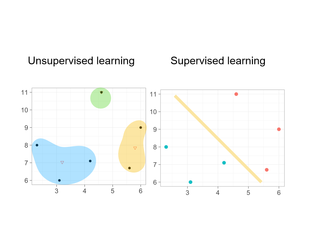
Unsupervised Learning

In unsupervised learning, the algorithm works with unlabeled data —there is no predefined target variable. The goal is to discover hidden patterns, structures, or groupings in the data.

Types of Unsupervised Learning:

1. Clustering:  Grouping similar data points together (e.g., customer segmentation). Examples: Market segmentation, anomaly detection, document categorization.
2. Dimensionality Reduction:  Reducing the number of features while preserving important information (e.g., PCA, t-SNE, UMAP). Examples: Data visualization, noise reduction, feature extraction.
3. Association Rule Learning:  Discovering relationships between variables (e.g., market basket analysis). Examples: Product recommendations, cross-selling strategies.

Common Algorithms:

• K-Means, Hierarchical Clustering, DBSCAN
• Principal Component Analysis (PCA)
• Autoencoders and Variational Autoencoders
• Apriori, FP-Growth (for association rules)

Business Example:

An e-commerce company uses clustering to segment customers based on browsing behavior, purchase history, and demographics. They discover five distinct customer personas and tailor marketing campaigns to each segment.

Semi-Supervised and Reinforcement Learning

• Semi-Supervised Learning:  Combines a small amount of labeled data with a large amount of unlabeled data. Useful when labeling is expensive.
• Reinforcement Learning:  An agent learns by interacting with an environment and receiving rewards or penalties. Used in dynamic decision-making (e.g., pricing algorithms, robotics).

9.3 The Machine Learning Project Lifecycle

Successful ML projects follow a structured lifecycle that aligns technical work with business objectives. The lifecycle is iterative, not linear—expect to revisit earlier stages as you learn more.

9.3.1 Problem Framing and Success Metrics

Problem Framing:
The first and most critical step is to clearly define the business problem and translate it into an ML task. Ask:

• What decision are we trying to improve?
• What would success look like?
• Is ML the right approach, or would a simpler solution suffice?

Examples of Problem Framing:

Defining Success Metrics:

Success metrics should align with business goals, not just technical performance. Consider:

• Business Metrics:  Revenue impact, cost savings, customer satisfaction, operational efficiency.
• Technical Metrics:  Accuracy, precision, recall, F1-score, RMSE, AUC-ROC.

Example:

For a churn prediction model, technical accuracy might be 85%, but the business metric is the reduction in churn rate  and the ROI of retention campaigns . A model with 80% accuracy that identifies high-value customers at risk may be more valuable than a 90% accurate model that flags low-value customers.

AI Prompt for Problem Framing:

"I work in [industry] and want to reduce [business problem]. What are potential ways to frame this as a machine learning problem? What success metrics should I track?"

9.3.2 Data Selection and Preparation

Data Selection:

Identify the data sources needed to solve the problem. Consider:

• Internal data:  CRM systems, transaction logs, operational databases.
• External data:  Market data, social media, third-party datasets.
• Data quality:  Is the data complete, accurate, and representative?

Data Preparation:

This stage often consumes 60-80% of project time. Key tasks include:

• Handling missing values and outliers (see Chapter 8).
• Encoding categorical variables.
• Feature engineering and transformation.
• Splitting data into training, validation, and test sets.

Avoiding Data Leakage:

Ensure that information from the future or the target variable does not leak into the training data. For example, if predicting customer churn, do not include features like "number of support tickets after churn date."

9.3.3 Model Training, Validation, and Tuning

Model Training:

Select appropriate algorithms based on the problem type, data characteristics, and interpretability needs. Start simple (e.g., logistic regression, decision trees) before moving to complex models (e.g., gradient boosting, neural networks).

Validation Strategy:

Use cross-validation to assess model performance on unseen data and avoid overfitting. Common strategies:

• K-Fold Cross-Validation:  Split data into K folds, train on K-1 folds, validate on the remaining fold, repeat K times.
• Time-Series Split:  For temporal data, use past data to predict future outcomes, respecting the time order.

Hyperparameter Tuning:

Optimize model hyperparameters (e.g., learning rate, tree depth, regularization strength) using techniques like:

• Grid Search - exhaustive search good for discrete values but time consuming if many parameters.
• Random Search - fasters
• Bayesian Optimization - Best if search space is very large

Example in Python:

from sklearn.model_selection import GridSearchCV
from sklearn.ensemble import RandomForestClassifier

param_grid = {
   'n_estimators': [50, 100, 200],
   'max_depth': [5, 10, 15],
   'min_samples_split': [2, 5, 10]
}

rf = RandomForestClassifier(random_state=42)
grid_search = GridSearchCV(rf, param_grid, cv=5, scoring='f1')
grid_search.fit(X_train, y_train)

print("Best parameters:", grid_search.best_params_)
print("Best F1 score:", grid_search.best_score_)

Model Evaluation:

Evaluate the final model on a held-out test set using appropriate metrics. For classification:

• Accuracy:  Overall correctness.
• Precision:  Of predicted positives, how many are correct?
• Recall (Sensitivity):  Of actual positives, how many did we catch?
• F1-Score:  Harmonic mean of precision and recall.
• AUC-ROC:  Area under the receiver operating characteristic curve.

For regression:

• RMSE (Root Mean Squared Error):  Penalizes large errors.
• MAE (Mean Absolute Error):  Average absolute error.
• R² (Coefficient of Determination):  Proportion of variance explained.

9.3.4 Deployment, Monitoring, and Maintenance

Deployment:

Move the model from development to production where it can make real-time or batch predictions. Deployment options include:

• Batch predictions:  Run the model periodically on new data (e.g., daily churn scores).
• Real-time API:  Serve predictions on-demand via a web service.
• Embedded models:  Integrate the model into applications or devices.

Monitoring:

Once deployed, continuously monitor model performance to detect:

• Data drift:  Changes in input data distribution over time.
• Concept drift:  Changes in the relationship between inputs and outputs.
• Performance degradation:  Declining accuracy or business metrics.

Example Monitoring Metrics:

• Prediction distribution over time.
• Feature distributions compared to training data.
• Business KPIs (e.g., conversion rate, revenue per prediction).

Maintenance:

Retrain models periodically with fresh data to maintain performance. Establish a feedback loop where model predictions and outcomes are logged and used to improve future iterations.

AI Prompt for Deployment Planning:

"What are best practices for deploying a [model type] model in a [industry] production environment? What monitoring metrics should I track?"

9.4 Overfitting, Underfitting, and the Bias–Variance Trade-off

Understanding overfitting and underfitting is crucial for building models that generalize well to new data.

Underfitting

Definition:  The model is too simple to capture the underlying patterns in the data. It performs poorly on both training and test data.

Symptoms:

• Low training accuracy.
• Low test accuracy.
• High bias.

Causes:

• Model is too simple (e.g., linear model for non-linear data).
• Insufficient features.
• Over-regularization.

Solutions:

• Use a more complex model.
• Add more relevant features.
• Reduce regularization strength.

Overfitting

Definition:  The model learns the training data too well, including noise and outliers, and fails to generalize to new data.

Symptoms:

• High training accuracy.
• Low test accuracy.
• High variance.

Causes:

• Model is too complex (e.g., deep decision tree).
• Too many features relative to data size.
• Insufficient regularization.
• Training for too many epochs (neural networks).

Solutions:

• Simplify the model (e.g., reduce tree depth, use fewer features).
• Apply regularization (L1, L2, dropout).
• Use more training data.
• Apply cross-validation.
• Early stopping (for iterative algorithms).

The Bias–Variance Trade-off

Bias:  Error from overly simplistic assumptions in the model. High bias leads to underfitting.

Variance:  Error from sensitivity to small fluctuations in the training data. High variance leads to overfitting.

Trade-off:  As model complexity increases, bias decreases but variance increases. The goal is to find the sweet spot that minimizes total error.

Visualization:

Total Error = Bias² + Variance + Irreducible Error

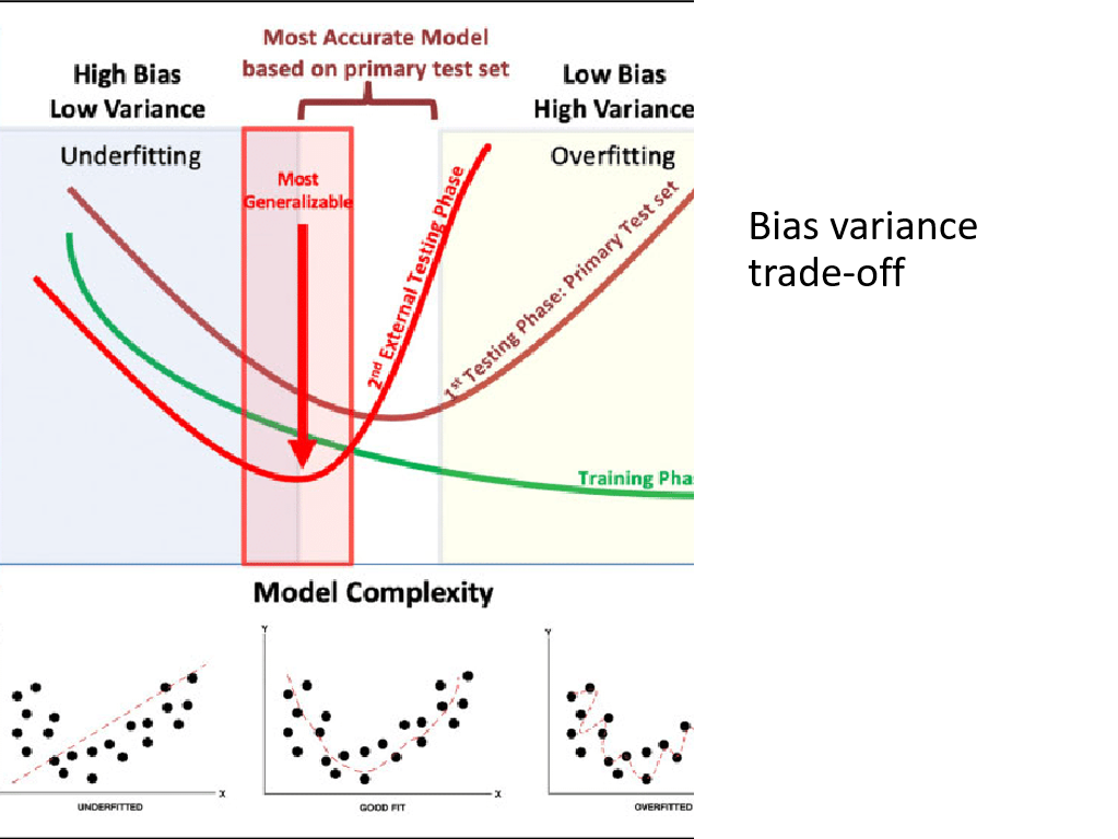
Underfitting        Optimal        Overfitting

(High Bias)         (Balanced)     (High Variance)

Example in Python:

import numpy as np

import matplotlib.pyplot as plt

import seaborn as sns

from sklearn.datasets import make_classification

from sklearn.model_selection import learning_curve

from sklearn.linear_model import LogisticRegression

# Seaborn style

sns.set_theme(style="whitegrid", palette="Set2")

# Create example dataset

X, y = make_classification(

    n_samples=1000,

    n_features=20,

    n_informative=15,

    n_redundant=5,

    random_state=42

)

# Model

model = LogisticRegression(max_iter=1000)

# Learning curve

train_sizes, train_scores, val_scores = learning_curve(

    model,

    X,

    y,

    cv=5,

    scoring="accuracy",

    train_sizes=np.linspace(0.1, 1.0, 10)

)

train_mean = train_scores.mean(axis=1)

val_mean = val_scores.mean(axis=1)

# Plot

plt.figure(figsize=(8, 5))

plt.plot(train_sizes, train_mean, marker="o", linewidth=2, label="Training score")

plt.plot(train_sizes, val_mean, marker="s", linewidth=2, label="Validation score")

plt.xlabel("Training Set Size")

plt.ylabel("Accuracy")

plt.title("Learning Curve")

plt.legend()

plt.tight_layout()

plt.show()

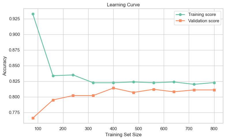
Interpretation:

• If both curves plateau at low accuracy: underfitting  (add complexity).
• If training accuracy is high but validation accuracy is low: overfitting  (reduce complexity or add data).
• If both curves converge at high accuracy: good fit .

9.5 Interpretability vs. Accuracy Trade-offs

In business analytics, model interpretability is often as important as accuracy. Stakeholders need to understand why  a model makes certain predictions to trust and act on them.

The Spectrum of Interpretability

Highly Interpretable Models:

• Linear Regression, Logistic Regression
• Decision Trees (shallow)
• Rule-based models

Advantages:  Easy to explain, transparent, auditable.
Disadvantages:  May sacrifice accuracy for simplicity.

Black-Box Models:

• Deep Neural Networks
• Gradient Boosting Machines (complex ensembles)
• Random Forests (large ensembles)

Advantages:  Often achieve higher accuracy.
Disadvantages:  Difficult to interpret, harder to debug, less trustworthy.

When Interpretability Matters

High Interpretability Needed:

• Regulated industries:  Finance, healthcare, insurance (e.g., credit decisions must be explainable).
• High-stakes decisions:  Medical diagnosis, criminal justice, hiring.
• Stakeholder trust:  Executives and domain experts need to understand model logic.
• Debugging and improvement:  Understanding errors helps refine models.

Lower Interpretability Acceptable:

• Recommendation systems:  Users care about quality, not explanation.
• Fraud detection:  Speed and accuracy matter more than explaining every flag.
• Image/speech recognition:  Inherently complex tasks where interpretability is less critical.

Techniques for Improving Interpretability

Even for black-box models, several techniques can provide insights:

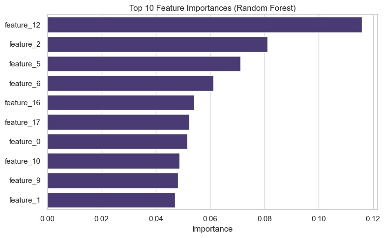
1. Feature Importance:

Identify which features contribute most to predictions.

import pandas as pd

from sklearn.ensemble import RandomForestClassifier

rf = RandomForestClassifier(n_estimators=100, random_state=42)

rf.fit(X_train, y_train)

importance = pd.DataFrame({

    'feature': X_train.columns,

    'importance': rf.feature_importances_

}).sort_values('importance', ascending=False)

print(importance.head(10))

# Plot top 10 feature importances

plt.figure(figsize=(8, 5))

sns.barplot(

    data=importance.head(10),

    x="importance",

    y="feature"

)

plt.title("Top 10 Feature Importances (Random Forest)")

plt.xlabel("Importance")

plt.ylabel("")

plt.tight_layout()

plt.show()

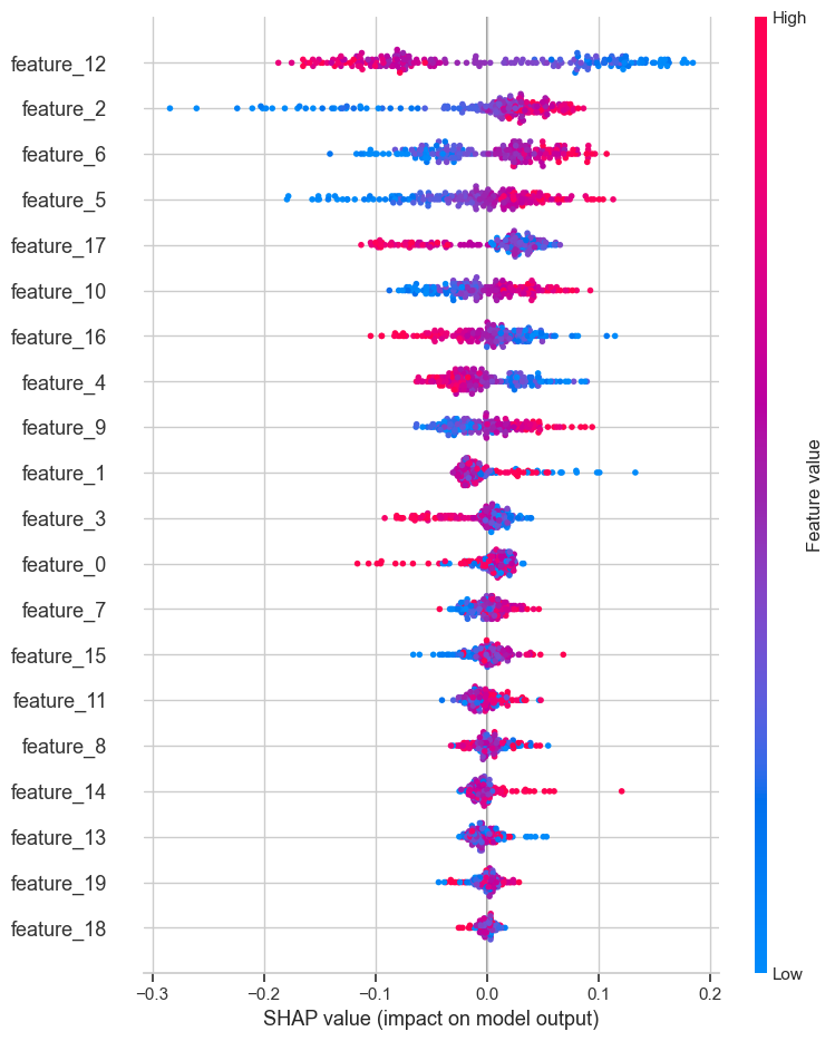
2. SHAP (SHapley Additive exPlanations):

Explains individual predictions by showing the contribution of each feature.

import shap
explainer = shap.TreeExplainer(rf)
shap_values = explainer.shap_values(X_test)
shap.summary_plot(shap_values[1], X_test)

3. LIME (Local Interpretable Model-agnostic Explanations):

Approximates the black-box model locally with an interpretable model.

4. Partial Dependence Plots:

Show the relationship between a feature and the predicted outcome, holding other features constant.

5. Model Simplification:

Use a complex model to generate predictions, then train a simpler, interpretable model (e.g., decision tree) to approximate it.

Balancing Accuracy and Interpretability

Strategy:

• Start with interpretable models as a baseline.
• If accuracy is insufficient, move to more complex models.
• Use interpretability techniques to explain complex models.
• Consider hybrid approaches:  Use a black-box model for predictions but provide explanations via SHAP or LIME.

Business Consideration:

A 2% gain in accuracy may not justify a complete loss of interpretability if stakeholders cannot trust or act on the model's recommendations.

9.6 Responsible and Fair ML in Business

Machine learning models can perpetuate or amplify biases present in training data, leading to unfair or discriminatory outcomes. Responsible ML practices are essential for ethical and legal compliance.

Sources of Bias in ML

1. Historical Bias:

Training data reflects past inequalities or discriminatory practices.

Example:  A hiring model trained on historical data may favor male candidates if the company historically hired more men.

2. Representation Bias:

Training data does not represent the full population.

Example:  A facial recognition system trained primarily on light-skinned faces performs poorly on darker-skinned faces.

3. Measurement Bias:

Features or labels are measured inaccurately or inconsistently across groups.

Example:  Credit scores may be less reliable for certain demographic groups due to limited credit history.

4. Aggregation Bias:

A single model is used for groups with different relationships between features and outcomes.

Example:  A medical diagnosis model trained on adults may perform poorly on children.

Fairness Metrics

Several metrics quantify fairness, though no single metric is universally appropriate:

1. Demographic Parity:

Positive prediction rates are equal across groups.

2. Equal Opportunity:

True positive rates (recall) are equal across groups.

3. Equalized Odds:

Both true positive and false positive rates are equal across groups.

4. Predictive Parity:

Precision is equal across groups.

Trade-offs:

It is often mathematically impossible to satisfy all fairness criteria simultaneously. Choose metrics aligned with business values and legal requirements.

Strategies for Fair ML

1. Audit Training Data:

Examine data for representation and historical biases. Collect more diverse data if needed.

2. Remove Sensitive Features:

Exclude protected attributes (e.g., race, gender) from the model. However, this does not guarantee fairness if other features are correlated with protected attributes (proxy discrimination).

3. Reweighting or Resampling:

Adjust training data to balance representation across groups.

4. Fairness-Aware Algorithms:

Use algorithms designed to optimize for both accuracy and fairness.

5. Post-Processing:

Adjust model predictions to satisfy fairness constraints.

6. Human Oversight:

Ensure human review for high-stakes decisions, especially when models flag edge cases.

Transparency and Accountability

Documentation:

Maintain clear documentation of:

• Data sources and preprocessing steps.
• Model architecture and hyperparameters.
• Performance metrics, including fairness audits.
• Deployment and monitoring procedures.

Model Cards:

Publish "model cards" that describe the model's intended use, limitations, performance across groups, and ethical considerations.

Regulatory Compliance:

Be aware of regulations like GDPR (Europe), CCPA (California), and industry-specific rules (e.g., Fair Credit Reporting Act in the U.S.) that govern automated decision-making.

AI Prompt for Fairness Auditing:

"How can I audit a [model type] model for fairness across demographic groups? What metrics and techniques should I use?"

Exercises

Exercise 1: Frame a Business Problem as a Supervised or Unsupervised Learning Task

Scenario:  You work for a telecommunications company experiencing high customer churn. Management wants to reduce churn and improve customer retention.

Tasks:

1. Frame this as a supervised learning problem. What is the target variable? What features might be relevant?
2. Frame this as an unsupervised learning problem. How would clustering help?
3. Which approach would you recommend and why?

Exercise 2: Sketch a Full ML Workflow for Credit Risk Scoring

Scenario:  A bank wants to build a credit risk scoring model to predict the likelihood of loan default.

Tasks:

1. Problem Framing:  Define the ML task (classification or regression?) and success metrics (both technical and business).
2. Data Selection:  What data sources would you use? List at least 5 relevant features.
3. Model Training:  Suggest 2-3 algorithms to try and explain why.
4. Validation:  What validation strategy would you use? What metrics would you track?
5. Deployment:  How would the model be deployed? What monitoring metrics are critical?
6. Fairness:  What fairness concerns might arise? How would you address them?

Exercise 3: Analyze Examples of Overfitting and Underfitting

Scenario:  You trained three models on a customer churn dataset. Here are the results:

Tasks:

1. Which model is likely underfitting? Explain.
2. Which model is likely overfitting? Explain.
3. Which model would you choose for deployment? Why?
4. What steps would you take to improve the underperforming models?

Exercise 4: Discuss Interpretability Needs for Different Stakeholders and Use Cases

Scenario:  Your company is deploying ML models for three different use cases:

1. Credit approval:  Deciding whether to approve a loan application.
2. Product recommendations:  Suggesting products to customers on an e-commerce site.
3. Predictive maintenance:  Predicting when factory equipment will fail.

Tasks:

1. For each use case, identify the key stakeholders (e.g., customers, regulators, operations team).
2. Assess the interpretability needs for each use case (high, medium, low) and justify your assessment.
3. Recommend a modeling approach for each use case, balancing accuracy and interpretability.
4. Suggest specific interpretability techniques (e.g., SHAP, feature importance) that would be most useful for each use case.

Chapter Summary:

Machine learning is a powerful tool for business analytics, but success requires more than technical skill. By understanding the ML lifecycle, recognizing the trade-offs between accuracy and interpretability, and committing to responsible and fair practices, business analysts can deploy models that create real value while maintaining trust and ethical standards. The exercises in this chapter challenge you to apply these concepts to realistic business scenarios, preparing you for the complexities of real-world ML projects.